This is the HTML version of a Mathematica 8/9 notebook. You can copy and paste the following into a notebook as literal plain text. For the motivation and further discussion of this program, see "Mathematica density and contour Plots with rasterized image representation". Use this function just as you would ListDensityPlot, except that you can also add options recognized by ListContourPlot. A usage example is given at the bottom of this page.
listContourDensityPlot[pList_, opts : OptionsPattern[]] :=
 (* //Created by Jens U.Nöckel for Mathematica 8,12/2011 *)
 Module[
{
pL,
p,
plotRangeRule,
img,
cont,
densityOptions,
contourOptions,
frameOptions,
rangeCoords
},
  densityOptions =
   Join[FilterRules[{opts},
     FilterRules[Options[ListDensityPlot],
      Except[{ImageSize,Prolog, Epilog, FrameTicks, PlotLabel, GridLines, Mesh, AspectRatio, PlotRangePadding,
        ImagePadding, Frame, Axes}]]], {PlotRangePadding -> None,
     Frame -> None, Axes -> None, ImagePadding -> None}];
  contourOptions =
   Join[FilterRules[{opts},
     FilterRules[Options[ListContourPlot],
      Except[{Prolog, Epilog, FrameTicks, Background, ContourShading,
        Frame, Axes}]]], {Frame -> None,
     Axes -> None, ContourShading -> False}];
  (* //The density plot img and contour plot "cont" are created here: *)
  pL = ListDensityPlot[pList, Evaluate@Apply[Sequence, densityOptions]];
  p=First@Cases[{pL},Graphics[__],\[Infinity]];
  plotRangeRule = FilterRules[Quiet@AbsoluteOptions[p], PlotRange];
  rangeCoords = Transpose[PlotRange /. plotRangeRule];
  img = Rasterize[p, "Image"];
  cont = If[
    MemberQ[{0, None}, (Contours /. FilterRules[{opts}, Contours])],
    {},
    ListContourPlot[pList,
     Evaluate@Apply[Sequence, contourOptions]]];
  (* //Before showing the plots, set the PlotRange for the frame which will be drawn separately:*)
  frameOptions =
   Join[FilterRules[{opts},
     FilterRules[Options[Graphics],
      Except[{PlotRangeClipping, PlotRange}]]], {plotRangeRule,
     Frame -> True, PlotRangeClipping -> True}];
  (* // To align the image img with the contour plot, enclose img
     // in a bounding box rectangle of the same dimensions as cont,
     // and then combine with cont using Show: *)
  If[Head[pL]===Legended,Legended[#,pL[[2]]],#]&@
  Show[Graphics[{
     Inset[Show[
       SetAlphaChannel[img, "ShadingOpacity" /. {opts} /. {"ShadingOpacity" -> 1}],
       AspectRatio -> Full],
      rangeCoords[[1]], {0, 0}, rangeCoords[[2]] - rangeCoords[[1]]]}, PlotRangePadding -> None], cont,
   Evaluate@Apply[Sequence, frameOptions]]
]
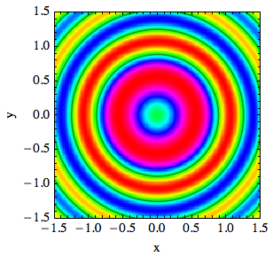
Here is an example of how to use the function:
listContourDensityPlot[
 Transpose@Table[Sin[4 (x^2 + y^2)]/Sqrt[x^2 + y^2 + .1], {x, -1.5,
   1.5, .05}, {y, -1.5, 1.5, .05}],
 DataRange -> {{-1.5, 1.5}, {-1.5, 1.5}}, Contours -> 2,
 PlotRange -> All, PlotRangePadding -> 0, ImageSize -> 200,
 FrameLabel -> {"x", "y"}, ColorFunction -> Hue,
 InterpolationOrder -> 2]
As with any ListDensityPlot, the smoothness of the false-color map depends on InterpolationOrder, ImageSize, and of course the number of data points.
By default, the image dimensions are scaled to yield the same tick mark spacing on both axes, but you can change this by specifying the option AspectRatio -> ratio, cf. the Mathematica documentation.
You can completely suppress the ListContourPlot output by giving the option Contours -> None.