This is the HTML version of a Mathematica 8/9 notebook. You can copy and paste the following into a notebook as literal plain text. For the motivation and further discussion of this program, see "Mathematica density and contour Plots with rasterized image representation". Use this function just as you would DensityPlot, except that you can also add options recognized by ContourPlot. A usage example is given at the bottom of this page.
contourDensityPlot[f_, rx_, ry_, opts : OptionsPattern[]] :=
 (* // Created by Jens U.Nöckel for Mathematica 8,revised 12/2011 *)
 Module[
{
img,
cont,
pL,
p,
plotRangeRule,
densityOptions,
contourOptions,
frameOptions,
rangeCoords
},
  densityOptions =
   Join[FilterRules[{opts},
     FilterRules[Options[DensityPlot],
      Except[{ImageSize,Prolog, Epilog, FrameTicks, PlotLabel, ImagePadding, GridLines, Mesh, AspectRatio,
        PlotRangePadding, Frame, Axes}]]], {PlotRangePadding -> None,
     ImagePadding -> None, Frame -> None, Axes -> None}];
  pL = DensityPlot[f, rx, ry, Evaluate@Apply[Sequence, densityOptions]];
  p=First@Cases[{pL},Graphics[__],\[Infinity]];
  plotRangeRule = FilterRules[Quiet@AbsoluteOptions[p], PlotRange];
  contourOptions =
   Join[FilterRules[{opts},
     FilterRules[Options[ContourPlot],
      Except[{Prolog, Epilog, FrameTicks, Background, ContourShading, Frame,
        Axes}]]], {Frame -> None,
     Axes -> None, ContourShading -> False}];
  (* //The density plot img and contour plot cont are created here: *)

    img = Rasterize[p, "Image"];
  cont = If[
     MemberQ[{0, None}, (Contours /. FilterRules[{opts}, Contours])],
      {},
      ContourPlot[f, rx, ry,
      Evaluate@Apply[Sequence, contourOptions]]
     ];
  (* //Before showing the plots,set the PlotRange for the frame which will be drawn separately: *)
  frameOptions =
   Join[FilterRules[{opts},
     FilterRules[Options[Graphics],
      Except[{PlotRangeClipping, PlotRange}]]], {plotRangeRule,
     Frame -> True, PlotRangeClipping -> True}];
  rangeCoords = Transpose[PlotRange /. plotRangeRule];
  (* // To align the image img with the contour plot, enclose img in a
     // bounding box rectangle of the same dimensions as cont,
     // and then combine with cont using Show: *)
  If[Head[pL]===Legended,Legended[#,pL[[2]]],#]&@
  Show[Graphics[{
     Inset[Show[
       SetAlphaChannel[img,
        "ShadingOpacity" /. {opts} /. {"ShadingOpacity" -> 1}],
       AspectRatio -> Full],
      rangeCoords[[1]], {0, 0}, rangeCoords[[2]] - rangeCoords[[1]]]},
    PlotRangePadding -> None], cont,
   Evaluate@Apply[Sequence, frameOptions]]
]
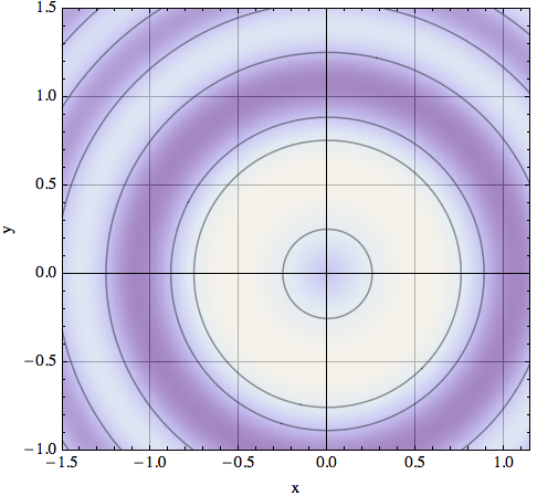
Here is a usage example:
contourDensityPlot[
 Sin[4 (x^2 + y^2)]/Sqrt[x^2 + y^2], {x, -1.5, 1.5}, {y, -1.5, 1.5},
 PlotPoints -> 60, PlotRange -> {{-1.5, 1.15}, {-1, 1.5}, {-5, 5}},
 Contours -> Automatic, Frame -> True, FrameLabel -> {"x", "y"},
 Axes -> True, "ShadingOpacity" -> .5, GridLines -> Automatic]
You can completely suppress the ContourPlot output by giving the option Contours -> None.
I also added an option "ShadingOpacity" that can be used to make the shaded background transparent. The shading is fully opaque for "ShadingOpacity" -> 1 and fully transparent for "ShadingOpacity" -> 0. This option is useful if you want to combine the plot with a Prolog, or if you have added Gridlines -> Automatic which usually will be hidden behind the density plot shading.