Graphics incompatibilities between Mathematica Versions

1. Should I be using Mathematica versions 8, 7, 6 or 5?

   Shortly after releasing version 6.03, Mathematica jumped to version 7. The transition from version 5 to 6 has greatly influenced the current content of this page, mainly because version 6 leaves a lot to be desired. More than ever, with the release of version 7, the bottom line is: do not use version 6. The simple reason is that V6 files may be incompatible with both V5 and V7. E.g., version 6 has no 3D arrows and is missing the Cone command (which exists in V5 and V7), and the syntax for BarChart is different in all three versions.

   What about version 5? It's definitely on the way out. On Mac OS X Snow Leopard, you can no longer move document windows with the mouse! This does not happen under Leopard, and it may be fixed at some point, but with the current state of affairs I would not recommend anyone use MMA 5.2. If you do have to use it (I sometimes have to), windows can be moved from within the notebook by using the following work-around:
   With[{x =100, y = 10}, SetOptions[EvaluationNotebook[], WindowMargins -> {{x, Automatic}, {Automatic,y}}]]
   Adjust the parameters x and y to get the desired space between the window and the left top corner of the screen.

   Within the graphics-oriented context of this page, the question therefore is not so much whether or not to use the latest version; in general, you should get the latest upgrades. However, there will be a learning curve both for new users and for version-5 users. Here is some information that I collected while approaching this transition.

   • If you're new to Mathematica, it is advisable to start with the latest version. The fundamentals of the language are quite stable, but the newest versions are likely to be more user-friendly. If you're coming to Mathematica from Wolfram Alpha (see above), version 8 has the advantage that the Alpha command line is also available from within the Mathematica notebook.

     If you're switching from version 5, you will learn to appreciate the ability of newer versions to automatically convert incompatible syntax. This process is imperfect, so you should probably step through the suggested changes one by one instead of accepting all changes blindly. That's also a good way to learn about the differences between old and new Mathematica syntax. Be sure to make a backup copy of any version-5 notebooks that you decide to convert to version ≥ 7.

     Here are some pointers that should help once you've mastered the introductory tutorials:

     • There is a "Virtual Book" similar to the old Mathematica book built into the help system of version ≥ 8. This should be the place to start.
     • Stephen Wolfram's "The Mathematica Book is written for version 5 but presents the main topics (such as the core language) in a coherent and readable form.
     • A good place to look for ideas is the Wolfram Demonstrations Project.
     • Another place to look, in particular for beginners, is the Mathematica Learning Center.
     • In everyday use, for quick help on a command (symbol), type ?Plot. Of course you may not always remember the name of a command. If you're looking for some plot command, type something like ?*Plot, or ?*Plot* if you want to include commands ending, say, in "Plot3D".
     • A good tutorial for the basics is "Mathematica Programming Fundamentals: Lecture Notes" by Richard Gaylord. The free book "Mathematica ® Programming - an advanced introduction" by Leonid Shifrin is an excellent advanced look at the programming language and some of its fundamental idioms, but does not focus on visualization.
   • The new features are nice for in-class demonstrations because a Mathematica notebook exposes the "guts" of functional evaluations while at the same time allowing interactive manipulation of the results.
   • On the other hand, for larger projects you don't really need interactive features, especially when they become unrealistically slow with large data sets.
   • With too much interactivity in a notebook, the Frontend starts feeling like a web page crowded with badly coded Java applets. After playing with this for a while, I much prefer my notebooks to be source-code oriented rather than GUI oriented.
   • Almost every half-way complex computation requires learning new or modified Mathematica syntax if you are switching from version 5.
   • Writing notebooks in Mathematica version 7, you lose backward compatibility, which may be a problem especially if your notebooks are intended for an audience who can't afford to upgrade from an earlier version yet.
   • In many situations, e.g., for documentation purposes, it is necessary to have static documents that preserve their content over time. With added interactivity, Mathematica notebooks may become less suitable for such purposes; in particular embedded graphics can now be modified by hand, without leaving a programmatic record in the notebook.
   • There is a vastly expanded range of image processing capabilities in Mathematica 7, which may allow users to consolidate the set of other tools they need to install. By comparison to other image processing software, Mathematica is however quite resource-hungry and slow, so that it will be hard to go beyond toy projects in Mathematica. See specifically the remarks on movies below.

   Bearing all this in mind, below are some things you may want to know when using Mathematica version ≥ 7. If you decide to stick with version 5, jump to the bottom of this page for hints that apply to all versions.

2. Avoiding Mathematica graphics incompatibilities between different versions

   From version 7 to version 8

   Mathematica 8 has been released, and it includes improvements in graphics, with a focus on three-dimensional plotting where currently there is a glaring under-utilization of the capabilities that most computers nowadays pack in their graphics cards. For example, texture mapping is finally be supported (that's the ability to project bitmap images onto the unwrapped surface of a 3D mesh; implemented in most 3D shaders and ray-tracers, e.g. OpenGL, POV-Ray and Blender). However, there are still bugs with the alpha channel, and the rendering model doesn't support true shadows.

   Although there are no incompatible changes listed on the official web site, I immediately had one incompatibility show up in a notebook written with version 7: Execute the following test: Mean@Flatten[First[ColorConvert[ExampleData[{"TestImage", "Lena"}], "GrayScale"]]]. It produces a number in MMA 7 but not in MMA 8. The reason is that the image data in the output of ColorConvert is stored as a "RawArray" in version 8, instead of a List as in version 7. This leads to a result that Mean can't handle. The problem is that by using First to extract the image data, I was relying on the internal structure of the image, which has changed in version 8. To avoid this, one should resort to the more high-level command ImageData; simply replace First by ImageData in the above example, and everything works (in MMA versions ≥ 6).

   From version 5 to version 6 and 7

   If you have old Mathematica notebooks (from version 5.2 or below) containing fancy graphics, then converting them to Mathematica Version 6 or 7 can be a lot of work. Don't expect all your graphics cells to be properly converted by the automated "version advisory" help that springs into action when you open an older notebook with a newer MMA version. In my experience, manual conversion is really unavoidable. Below I give a work-around, but I recommend relying on it only in emergencies when you need to produce quick results with older notebooks and don't have the time to worry about manual conversion to MMA 7:

   Put the following at the beginning of such notebooks:
   If[$VersionNumber >= 6., <<Version5`Graphics`,  <<Graphics`Graphics`; <<Graphics`Graphics3D`]
   Doing this (or some variation on the above), old notebooks become useable, in particular 3D graphics and animation where the transition to Version 6 has brought deep changes. See (e.g.), the list of incompatible changes at Wolfram.com, and in particular the changes to the 2D graphics and the 3D graphics systems.

   The If[$VersionNumber >= 6.,...] statement above is intended to make the notebook work in all versions of Mathematica, but this may need tweaking depending on your content (in particular the add-on packages you're calling). Most importantly, the notebook has to be authored and saved in version 5.x, because V 6 doesn't have an option to save in "V 5" - backward compatible format, and trying to load a V 6 notebook into Mathematica V 5 typically results in a crash.

   By loading <<Version5`Graphics`, you give up the main new features of version 6 and 7 graphics. But more importantly, there appears to be no programmatic way to save the resulting graphics as external files (EPS, PDF, PNG, etc.). You'll have a working notebook, but version 6 will silently refuse to Export pictures from it (low-level functions like Display don't seem to work either), leaving you with only two options:

   1. Click on the Image in the notebook, and copy it. Then open Preview or a similar graphics application and paste the Image from the clipboard. In Mathematica version 7, this seems to work nicely. It creates vector-graphics output.
   2. Take a screen shot. This of course creates a resolution-dependent bitmap.

   Switching back from V 5 to V 6 graphics is done by entering <<Version6`Graphics`. Unfortunately, after this switch, the graphics you produced with the old graphics commands are likely to produce errors whenever you try to process them further.

   Below I address some specific compatibility issues as I encounter them. Some points may help write notebooks that are compatible with both version 5 and 6. However, in many cases it will not be practical to make such "fat" (multi-version) notebooks. Instead, you'll probably end up writing separate notebooks for each version, as needed.

   • Plot labels with complex formatting

     Shown below is a simple plot, executed first in Mathematica V. 5 (left) and then in V. 6 (right)
     
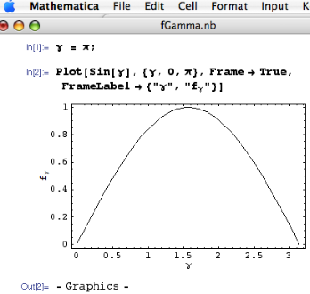
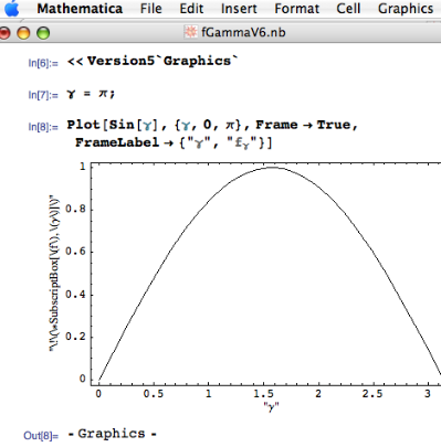
     In the Notebook, I used the symbol γ as a variable, but also as a frame label. In the label, I use "γ" in quotation marks to avoid getting the evaluated value of the variable γ as the horizontal label. Similarly, I quoted the symbol for the vertical label. So far, so good. But in version 6, the same method doesn't give the expected results, even though I've activated Version5`Graphics`. Not only do the quotation marks appear in the frame labels, but moreover the expression f_γ is not displayed as it should be. Everything works fine if I use Mathematica V. 6 without Version5`Graphics`.

     How can the frame labels be written in such a way that they display properly in both version 5, and version 6 with (or without) Version5`Graphics`? The solution is to use the following plot command instead:
     Plot[Sin[γ], {γ, 0, π}, Frame -> True, FrameLabel -> {HoldForm[γ], HoldForm[fγ]}]
     If we want our labels to be compatible with old and new versions of Mathematica, this is a way to do it.

   • 3D plotting functions and shadows

     In Mathematica version 6.0.3, some 3D plotting functions from the legacy add-on package Graphics3D have not yet been incorporated into the System context. For example, this applies to

     • Shadow
     • ShadowPlot3D
     • StackGraphics
     • ...
     The <<Version5`Graphics` trick won't bring them back, either. To accesss these functions, we have to load the Graphics3D add-on package in V 6. If you plan on using none of the new graphics features of V 6, you could just do the following:
     If[$VersionNumber >= 6., <<Version5`Graphics`,  <<Graphics`Graphics`];
 <<Graphics`Graphics3D`
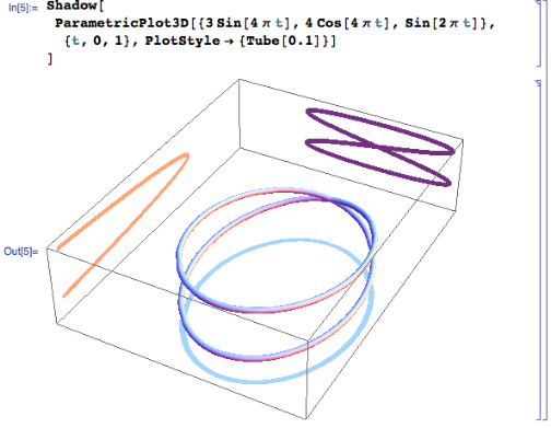
     Although this produces more warnings, it gets those shadow plots working properly.

     On the other hand, if you follow this route, you won't be able to run the command shown in the picture on the right. It uses a new V 6 feature, the Tube directive. In earlier versions of Mathematica, the command ParametricPlot3D creates one-dimensional lines that make it difficult to visualize complex 3D curves such as knots. Mathematica Version 6 now lets you choose a tube of user-specified diameter to represent the curve. The example plot uses the code
     Shadow[
ParametricPlot3D[{3 Sin[4 π t], 4 Cos[4 π t], Sin[2 π t]}, {t, 0, 1}, PlotStyle -> {Tube[0.1]}]
]
     You'll get an error here, unless we abandon the  <<Version5`Graphics`. I.e., you should only include the line
      <<Graphics`Graphics3D`
     This combines the best of the V 5 and V 6 worlds, in that the resulting curve is tubular with projections, and can even be interactively rotated. As of November 2008, Wolfram in fact offers slightly modified versions of the Graphics3D and Graphics add-on packages for downoad. See the Library pages for the Graphics`Graphics3D` and Graphics`Graphics` Legacy Standard Add-On Packages. However, I have been fine with the versions of the packages that are included in Mathematica.

     If you're willing to abandon the old commands (StackGraphics etc.) and replace them with functionally identical but syntactically more complex work-arounds, follow the compatibility instructions at the Wolfram site.

     The Shadow command won't work with version 8's Texture feature. For example, let's say you have a texture with an Alpha channel that produces transparent regions in the faces of a polygon. In a shadow plot, such holes of course should be reproduced as well — but they aren't. Mathematica's way to produce "shadows" is not at all related to the way shadows are produced in ray tracers (for comparison, see e.g. my notes on how to get shadows from a partly transparent texture in Blender). Instead, MMA simply squishes a copy of the 3D object to a really thin pancake in the projection direction. So there doesn't have to be an actual surface onto which the shadow falls, and the shadow itself is actually a 3D object with all the complexity of the original.

     I have written a function that uses the above technique to create shadows as projections of an object onto an arbitrarily tilted plane: planarShadow, listed here with an example. You can use this to re-create the above ShadowPlot3D, too.