Introduction — Obtaining Mathematica at the UO
Mathematica runs on many platforms, including Mac OS X. This page is written from a Mac OS X perspective, but if you're on a different platform you may still get some useful information here. In the past, I've also heavily used Mathematica on UNIX and Windows systems, and you shouldn't have any trouble adapting what I'm writing here to those other platforms. However, I have to leave that as an exercise for the reader. I'm trying to keep this page in step with changes in Mathematica, but the process of catching up with the most recent versions is still an ongoing effort.
Of course, if you need real expert help, you could always check one of these resources:
To obtain Mathematica through the University of Oregon site license, first check the information provided by IT Services. If you're a student planning to install Mathematica on your own computer, click on "Login to view available downloads" (bootom of page) and log in with your UO email address. Otherwise, do this:
To calculate with Mathematica within your web browser, use one of these online tools:
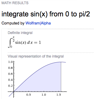
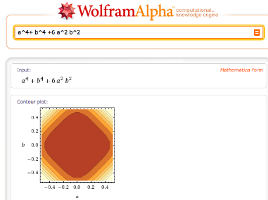 Although the graphics output is not (directly)
customizable, this is a very convenient way to get quick
plots from expressions in Mathematica syntax!
Wolfram Alpha can understand even
non-Mathematica syntax, and it does more than just
integrate and plot functions. It answers some math
questions better than Mathematica: e.g.,
Alpha supplies links to additional
information related to the functions it encountered in the
calculation.
Although the graphics output is not (directly)
customizable, this is a very convenient way to get quick
plots from expressions in Mathematica syntax!
Wolfram Alpha can understand even
non-Mathematica syntax, and it does more than just
integrate and plot functions. It answers some math
questions better than Mathematica: e.g.,
Alpha supplies links to additional
information related to the functions it encountered in the
calculation.
Alpha is continually improving, but Alpha is not a substitute for Mathematica. Computations that require complicated definitions and processing cycles will not be appropriate for Alpha.
 W|A
is integrated into the search engine "Bing" - but not
into Google. You can also install W|A
as an
iGoogle Gadget or Chrome Extension (among other things).
W|A
is integrated into the search engine "Bing" - but not
into Google. You can also install W|A
as an
iGoogle Gadget or Chrome Extension (among other things).
For more trivial tasks involving only basic algebra and
standard functions, Google already has a calculator
built-in. It is invoked whenever you enter something like
3.5*sin(0.5) in the web search box (the same
is true for Bing).
Sophisticated, automatically generated graphical output from nearly free-form natural language input
is one of the most interesting aspects of
Alpha. But don't expect W|A
to be a complete encyclopedia. Looking for the dielectric constant of water? Yes,
you get a number. But you also get a number (42) when
asking what the meaning of life is. And in both cases the
number alone leaves you somewhat dissatisfied because it
lacks context (incidentally, why is the dielectric constant
of water nearly twice the meaning of life?). Or, to quote
the Alpha web site:


 I have written a function that uses the above technique to create shadows as projections of an object onto an arbitrarily tilted plane: planarShadow, listed here with an example. You can use this to re-create the old ShadowPlot3D, too. With the function
 planarShadow from that page, the ominous bunny is created like this:
data = ExampleData[{"Geometry3D", "StanfordBunny"},
  "VertexData"]; bunny =
 ListSurfacePlot3D[data, MaxPlotPoints -> 50, Boxed -> False,
  Axes -> None, Mesh -> False];
z0 = Min[data[[All, 3]]];
Show[bunny, planarShadow[bunny, z0 {2, -11, 1}, {0, 0, 1}]]
 It's possible to use Mathematica as a
3D modeling tool, in particular when dealing with shapes
that are created and positioned programmatically. In
earlier versions (below 6), this requires loading various
packages to be able to specify standard shapes, rotate
objects etc. (
It's possible to use Mathematica as a
3D modeling tool, in particular when dealing with shapes
that are created and positioned programmatically. In
earlier versions (below 6), this requires loading various
packages to be able to specify standard shapes, rotate
objects etc. (Geometry`Rotations`,
Graphics`Shapes`,
Graphics`Polyhedra`,...) In Mathematica 6 and
up, much of this can be done without loading additional
packages.
The Cylinder command has become more
flexible, and a built-in command for drawing a 3D
arrow was introduced in
version 7; but it has some "quirks". E.g.,
here is what you get with Graphics3D[Arrow[Tube[{{0,
0, 0}, {1, 0, 0}}, Scaled[.05]]]]:  (yes, there is an arrowhead hidden in the hole
because it didn't scale with the tube). To fix this, the
arrowhead has to be scaled separately, like so:
(yes, there is an arrowhead hidden in the hole
because it didn't scale with the tube). To fix this, the
arrowhead has to be scaled separately, like so:
Graphics3D[{Arrowheads[.2],Arrow[Tube[{{0, 0, 0}, {1,
		  0, 0}}, Scaled[.025]]]}]
. This syntax requires some
care: the length in Arrowheads[.2] is a
scaled quantity relative to the size of the
graphic. The length determining the radius of the
Tube, however, must be written as
Scaled[.025] to have the same relationship to
the graphic dimensions. If you inadvertently type
both length scales the same way by entering
Arrowheads[Scaled[.2]], Mathematica version 7
will initially show no output, and then crash when you try
to correct the mistake. An additional directive
that you may want to group with the Arrow
command is CapForm["Butt"].
Presumably many users have devised their own 3D arrows in version ≤ 5, and none of these are likely to work with Mathematica 6 and above. As an illustration for how things work in version 6, here is my way of making an arrow. It requires no added packages, and scales the arrow head relative to the arrow thickness, not independently of it.
arrowLine[{p1_, p2_}, radius_:.1, headScale_:3] :=
 (* p1 and p2 are 3D points. They are passed as a list, to conform with the version-6 syntax for Cylinder[] *)
 Module[{p3, scale2, norm, pyramidHeight = 3/2},
  scale2 = headScale*radius;
  norm = Norm[p2 - p1];
  If[norm > scale2*pyramidHeight,
   p3 = p1 + (p2 - p1)/norm (norm - scale2 pyramidHeight);
   {
    EdgeForm[],
    Cylinder[{p1, p3}, radius],
    GeometricTransformation[
     GraphicsComplex[{{0, 0, pyramidHeight}, {0, -1, 0}, {0, 1, 0}, {-1, 0, 0}, {1, 0, 0}},
      Polygon[{{3, 4, 1}, {4, 2, 1}, {2, 5, 1}, {5, 3, 1}, {5, 2, 4, 3}}]],
     Composition[
      TranslationTransform[p3],
      Quiet[
       RotationTransform[{{0, 0, 1}, p2 - p1}], {RotationMatrix::degen, RotationTransform::spln}],
      ScalingTransform[scale2 {1, 1, 1}]]
     ]
    },{}
   ]]
The head is intentionally made of few polygons to limit memory usage when drawing a large number of arrows (and because the orientation of corners in the arrowhead can convey additional visual information).
The first argument is the pair of start and end points. The
two last arguments [optional] are the cross-sectional radius of the
arrow stem and the size of the arrowhead, as a multiple of the
radius. The default values are 0.1 for the radius and 3 for the
relative scale of the arrow head. The module returns a list that
can be displayed with a statement like
Graphics3D[arrowLine[{{0,0,0},{1,0,0}}]]. If the
arrow is too short compared to the head, an empty list is returned
which displays as nothing.
Click on this link to open a Notebook (PlaneWaveField.cdf) that illustrates the use of such vector drawings in electromagnetism (in particular showing polarization rotation in the Faraday effect).
Note: Since Mathematica version 7, there are the new functions VectorPlot3D and ListVectorPlot3D, which also let us draw 3D arrows using the option VectorStyle->"Arrow3D". You can also define your own arrow heads in those plots, as in VectorStyle -> Graphics3D[{EdgeForm[], GraphicsComplex[{{tipHeight, 0, 0}, {0, 0, -1}, {0, 0, 1}, {0, -1, 0}, {0, 1, 0}}, Polygon[{{3, 4, 1}, {4, 2, 1}, {2, 5, 1}, {5, 3, 1}, {5, 2, 4, 3}}]]}], where tipHeight=2 (e.g.). However, there seems to be no way to scale the thickness of the cylindrical shaft independently of its length.
If you do define your own vector plots as I did, but prefer smooth round arrows to my definition above, you can try the newly available standard 3D arrows (see image on the right) as in Graphics3D[{Arrowheads[.2], Arrow[Tube[{{0, 0, 0}, {0, 0, 1}}, .01]]}, Method -> {"TubePoints" -> 3, "ConePoints" -> 4}]. The Method option here is important when you need to speed up the rendering; default settings will make interactive 3D rotation feel sluggish when the number of arrows is large.
Instead of using an array of arrows to visualize three-dimensional vector fields, it can be more informative to display the field lines. These are one-dimensional curves whose tangent vectors are everywhere parallel to the given field. Such a representation is clearly useful when the field describes a physical flow of some kind, but it is also often used in electromagnetism. In 2D, Mathematica provides this plotting functionality in the function StreamPlot. For 3D fields, the function fieldLinePlot described on the linked page attempts to do the same thing.
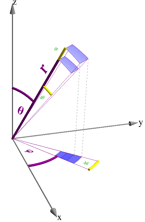
Axes labels in Mathematica's 3D plots always try to adjust themselves so as to face the reader. This is often quite nice, but it also means that the author doesn't have definitive control over the label orientation at the time the graphic is produced.
In a recent discussion on the Mathematica users group, I posted a relatively compact way of putting textual labels into a 3D plot in such a way that they are themselves Graphics3D objects that can subsequently be rotated, translated etc. An improved version of that function is discussed on the linked page, "Labels in Mathematica 3D plots".
This function requires MMA version 8. It can be invoked with any expression as the first argument, so it can also be used to embed 2D graphics into a Graphics3D (essentially a rasterized version of StackGraphics).
The picture on the right shows an application of these labels from a past lecture where I was illustrating spherical coordinates. The purple labels are created with the new function, the others are the standard type. The difference between these two types of labels is that the purple ones share the three-dimensional orientation of the object they refer to.
In 2D plots, it isn't always easy to accurately read off data by eye. In all earlier versions of Mathematica, you can examine the numerical values corresponding to positions in your plot by highlighting the graphic, then pressing Command. The current mouse position then appears at the bottom left of the Notebook window. You can click the mouse to make marks, and even copy marked coordinates by pressing Command-C.
In Mathematica ≥ 6, this must be done
differently.
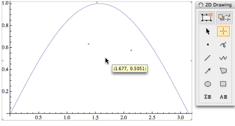
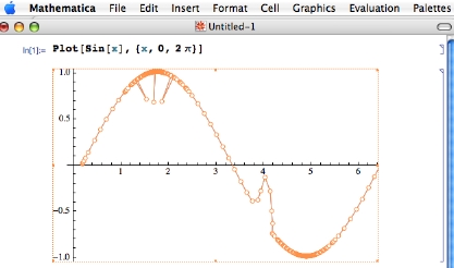
To get almost the same functionality as in version 5,
you first click on the image, then press
the period (. key), to get a cursor looking
like a cross-hair (it incorrectly appears as a normal
cursor in the screenshot). Also shown is the drawing
tools pallette that contains this function; it's activated
by pressing Ctrl-t.
The orange dots under the curve are marked coordinates, and the
hovering coordinate display follows the mouse.
 In
In
Mathematica 7 and above, additional functionality
has been added. See
the
video tutorial. There are some other interesting
features that appear in the detailed description ("More
Information") under
CoordinatesToolOptions: The options
"DisplayFunction" and
"CopiedValueFunction".
You may want to play with these options for several
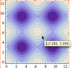
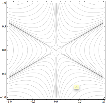
reasons. One is illustrated in the screen shot on the
left. First note that the ContourLabels
option has changed its meaning in version 7 from version 6,
and the documentation does not reflect
this: the choice Automatic now plots
no labels, but makes tooltips appear over the
contour lines. Here I was trying to see the value of a
contour from ContourPlot[Cos[x] + Cos[y], {x, 0, 4
Pi}, {y, 0, 4 Pi}, ContourLabels -> Automatic],
but at the same time tried to see the (x,y) coordinates.
But there is a conflict between the two floating boxes, in
that the coordinate display partly or completely obscures
the tooltip containing the contour height! It would be nice
to be able to control the justification of the tooltips,
but as an alternative one could do the
following:
f[x_, y_] := Cos[x] + Cos[y];
        ContourPlot[f[x, y], {x, 0, 4 Pi}, {y, 0, 4 Pi},
        CoordinatesToolOptions -> {"DisplayFunction" ->
        (Append[#,f @@ #] &)}]
With this, you get all three numbers in a single "Get
Coordinates" tooltip. Of course this is only worth doing if
the function value can be calculated quickly, but it can be
done equally well for DensityPlot,
e.g.
Alternatives for real-time display:
A real-time coordinate
display can also be produced using dynamic
interactivity. In particular, enter the following anywhere
in the Notebook:
Dynamic[MousePosition["Graphics"]]
and the result is a continuously updated mouse position,
whenever you hover over a plot. The coordinates here are
those of the graph's PlotRange. If the option
"Graphics" is omitted, the coordinates are
referenced to the Notebook window.
You can even get almost the old (version-5) behavior back
by drawing your graphics using the StatusArea
command, as shown in this example from the
documentation:
Dynamic[StatusArea[Plot[Sin[x], {x, 0, 10}],
        MousePosition["Graphics"]]]
Of course, this may eventually only have sentimental value
since the coordinates in the status area are actually
harder to read than a normal Notebook line.
Alternatives for coordinate copying:
Arguably a more useful operation is to actually copy and
save the mouse coordinates at selected points in the plot.
To get a snapshot of the mouse coordinates in the graph
every time the mouse is clicked, enclose all
plotting commands in a ClickPane directive,
e.g.,
ClickPane[ Plot[Cos[x], {x, -π, π}, Frame ->
        True, FrameLabel -> {α, "cos α"}], (pt = #)
        &]
which will update the variable pt at every
mouse click in the plot. Now you have to dynamically
display this variable somewhere in the Notebook:
Dynamic[pt]
That captures the desired coordinates.
If you don't want to re-evaluate the expression that draws your plot, just to make it clickable, there is a more indirect way:
ClickPane[, (pt = #) &]. This
is what it might look like: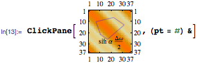
Dynamic[pt]
How accurate the coordinates are that you picked in the above approaches depends on how well you can position the mouse. However, in some cases, such as ListPlot, you may want exactly the coordinates of a discrete data point, even when you only manage to click somewhere in its neighborhood. The simplest way to do this is to wrap the data list in Tooltip to get a floating display of the data coordinates, similar to what I showed in the ContourPlot example above. But that doesn't let you easily copy the coordinates from the tool tip.
For such cases, we can "augment" the Tooltip functionality by piggy-backing a PopupWindow on each of the Tooltip instances contained in the plot. This requires one simple replacement rule:
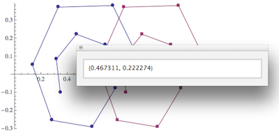
toolRule=Tooltip[x__]:>PopupWindow[Tooltip[x],Last[{x}]];
which can be appended to any plot (or arbitrary expression) to convert simple Tooltips into clickable popup windows. For example, here is a plot of two data sets, illustrating how you would simply wrap all the data in a single Tooltip first, and then apply my rule:
ListPlot[Tooltip@Evaluate[
 Table[N@Table[p+Exp[-t/10] { Cos[t],Sin[t]}/2,{t,0,10,1}],
   {p,{{.5,0},{1,0}}}
   ]],
  Joined->True, PlotMarkers->Automatic
]/.toolRule
The resulting plot is shown in the screen shot, after clicking one of the data points.
The main problem can be summarized in one word: speed.
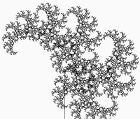
I just looked at one of the featured (May 2011) interactive demonstrations at
demonstrations.wolfram.com: "TreeBender." It's a nice interactive fractal tree. But it appears to be only a minor adaptation of another online demo that has, since 2010, been one of the all-time favorites at openprocessing.org: "Advanced Tree Generator," created by my son James Nöckel in Processing, a Java-based language. Compare for yourself which of these demos runs more smoothly and feels more responsive (James implemented a delay for more physical, smooth response, and you can crank up the number of branchings much higher). There are more dramatic examples, but the message is: Java, Flash and (lately) even Javascript can often beat Mathematica when interactivity is required.
You will notice speed issues as well when you try my above Clickpane[]
suggestion with a reasonably large plot, containing so many
data points that it takes a perceptible time to draw. The
mouse clicks will then be registered with an annoying time
delay. This is, I think, a real stumbling block in
data-intensive applications. To boil this issue down to its
core, I've tried the following simple experiment: Copy the
following code into two Mathematica Input lines:
x = Dynamic[MousePosition[]]
{ListPlot[
  Evaluate[
   Table[{.5, 0} + Exp[-t/100] {0.5 Cos[t], 0.5 Sin[t]}, {t, 0, 100, .001}]],
  Frame -> True], x}
This may take a second or two to generate the graph of a
dense spiral. The main thing to observe here is the
displayed mouse position: Its coordinates are updated very
sluggishly, both in the Out[] line of the assignment
x = , and in the Out[] line containing the
graphics object together with the value of x
in a list.
Now edit the above input so that the graphics
object does not appear combined with the current
mouse position, by changing the x at the very
end to "x". Note that the Mouse position
displayed as the first output line is now much more
responsive.
There is absolutely no difference between the graphics objects I am defining in either case, but the mere fact that the dynamic variable shares the same output cell as the graphics object in the first example causes a dramatic slow-down of the user interface. The delay doesn't seem to be caused directly by a redundant redrawing of the graphics object, but the Front End event handling is clearly inefficient. I'm currently waiting to hear back from Wolfram's experts on this; stay tuned.
The focus here is on exporting as PDF or
EPS.
Many Mathematica graphics functions use
VertexColors, a feature which is not
supported by all but the most recent versions of
PDF. To avoid difficulties with external
applications, export such graphics by selecting them,
then choosing the menu item File > Save
Selection As..., and opening the
Options dialog. There, choose "Use bitmap
representation" for graphics containing smooth shading.
Alternatively, export directly to a bitmap format such
as PNG.
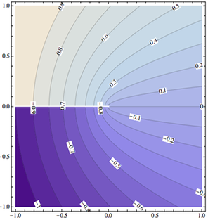
 In
Mathematica 5.2, the command
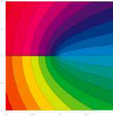
In
Mathematica 5.2, the command im0
= ContourPlot[Im[(x + I y)^(1/2)], {x, -1, 1}, {y, -1,
1}, Contours -> 21, PlotPoints -> 200,
ColorFunction -> Hue] produces the
illustration shown on the left. The shaded areas
are made from stacks of uniformly colored shapes, and
their number is of the order of the number of contours.
There is no degradation in quality when exporting this
plot.
However, in Mathematica 6, 7 and 8,
you may see something quite ugly if you create a plot
like im1 = ContourPlot[Im[(x + I y)^(1/2)], {x,
-1, 1}, {y, -1, 1}, Contours -> 20]: in
the exported EPS or
PDF, 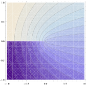 you get
something that looks as if it has been put together as
a 1000-piece puzzle, with white lines crisscrossing the
shaded areas,
see the screenshot on the right.
you get
something that looks as if it has been put together as
a 1000-piece puzzle, with white lines crisscrossing the
shaded areas,
see the screenshot on the right.
This is because the polygons defining the shaded
areas have invisible edges, and don't quite overlap.
The large number of polygons is a clear step backwards
compared to version 5.2, but at least the "puzzle
piece" artifact can be removed by giving the edges the
same color as the polygons. Here is a command that
makes the necessary replacement, and then exports to
PDF:
Export["plot.pdf", im1 /. {EdgeForm[],
            r_?(MemberQ[{RGBColor, Hue, CMYKColor, GrayLevel},
            Head[#]] &), i___} :> {EdgeForm[r], r,
            i}]
The file exported as "plot.pdf" no longer shows
the white lines and presents a contiguous,
smooth appearance.
If you also need to apply this trick to the graphics in
the notebook itself, then it may be convenient to
define a rule once and for all:
contourPlotRule=({EdgeForm[],
            r_?(MemberQ[{RGBColor, Hue, CMYKColor, GrayLevel},
            Head[#]] &), i___} :> {EdgeForm[r], r,
            i});
Then you can type the shorter expression im1/.
contourPlotRule to get an improved shading.
If the artifacts still aren't quite gone after applying the above
rule, you may want to add one more thing:
contourPlotRule=({EdgeForm[],
            r_?(MemberQ[{RGBColor, Hue, CMYKColor, GrayLevel},
            Head[#]] &), i___} :>
            {EdgeForm[{r,Thickness[Small]}], r, i});
This sets the edge thickness just large enough to avoid
the empty spaces between tiles.
I even had the crisscross artifacts appear on screen
on one of my Mathematica installations. This problem was fixed as follows: Quit Mathematica and move the user directory ~/Library/Mathematica out of the way. After relaunching Mathematica, this directory was rebuilt and the issue disappeared.
The root cause of the puzzle-piece artifacts is the large number of triangles with which Mathematica represents contour shading and density plots.
 This in itself is a problem that can come back to bite you in an external graphics program because it not only increases the exported file size but also makes it slow to render. On the right is a snapshot I took in Illustrator while resizing a
 PDF produced with the following command:
ContourPlot[
 Sin[4 (x^2 + y^2)]/Sqrt[x^2 + y^2], {x, -1.5, 1.5}, {y, -1.5, 1.5},
 PlotPoints -> 60, PlotRange -> {{-1.5, 1.15}, {-1, 1.5}, {-5, 5}},
 Contours -> 1, Frame -> True, FrameLabel -> {"x", "y"}, Axes -> True]
To create a PDF that is four times smaller and renders much faster, I wrote a different plotting function contourDensityPlot that superimposes a contour plot on the rasterized version of a density plot. See the definition and an example here. It should accept most of the options that DensityPlot and ContourPlot understand.
For more information, see this separate page:
"Mathematica density and contour Plots with rasterized image representation"
Mathematica V. 6 has introduced the ability to
create opacity effects, both in 2D and in 3D
graphics. Transparent portions can be useful in
Mathematica graphics because they let you display
several objects without having them obscure each other.
A simple example in 2D plots are intesecting areas such
as those created by the Filling option. In
3D, surfaces with opacity less than one let us reveal
axes and other objects that might otherwise be
obscured.
That's all very well as long as you're content with Mathematica itself as the vehicle for disseminating your work. But normally this isn't where you'd want to stop. You'd go on to export your graphics for inclusion in some other media, e.g. PDF or HTML, or for post-processing in a graphics program.
What happens to transparency then?
For the most part, what you really want is for the graphic to look the same in the external application as in your Mathematica Notebook. That means, once opacity has done its job of revealing various hidden things in your Mathematica plots, there is no need for the exported graphic to "remember" that it came from a partly transparent object. In that case you'll be fine choosing any export format that's convenient, making sure to think twice about using vector formats when exporting 3D graphics (because the files can get huge).
Things get a bit more difficult if you insist on maintaining transparency as a property of the exported graphics. There are not too many formats that support this.
The most well-known bitmap format that
does this is GIF, but one can also use PNG or TIFF
instead. Not among the eligible formats is
the popular JPEG. In Mathematica, GIF is
the most flexible choice, because it supports the
option TransparentColor. Here is the
syntax:
Export["plot.gif", Style[%, Magnification
                -> 2], "TransparentColor" ->
                White]
If you want to get a transparent
PNG or TIFF, replace the
option "TransparentColor" -> White
above by Background->None.
Alternatively, if transparency is desired for other
parts of the image, you could first use the command
Export["plot.png", Style[%, Magnification
                -> 2]]
(version-6 syntax), and then
process the result along the lines of the notes on
transparency in
bitmap graphics. The option Magnification
-> 2 magnifies graphics including plot
labels, whereas an option such as ImageSize
-> 600 makes the plot labels look smaller
compared to the graphics. More on Magnification
below.
As for vector formats, the good old EPS
format is out when transparency is desired. But you
can export as PDF or as
SVG. Since PDF is the
most familiar one, that may be preferred by many.
If you open such a PDF in Illustrator, it will
retain the opacity settings from Mathematica.
You don't see that at first, though,
because the PDF is by default exported with a solid
background. To get the transparent appearance back,
export your plot as follows:
Export["plot.pdf", Style[%, Background ->
                None]]
(V 6 syntax).
For completeness: you can remove the background in
version 5 PDFs, too, by typing
Export["plot.pdf", %, ConversionOptions ->
                {"Background" -> None}]]
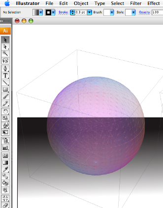
The picture on the right shows a
Mathematica-generated PDF, with a
black gradient added in Illustrator to show that
the sphere is translucent.
If you choose SVG export, then the
default is to include no background, so there's no
additional step involved. The disadvantage of SVG
is mainly the lack of full support for its
specification in many graphics editors and
browsers. Adobe Illustrator does a good job with
SVG, but for complex SVG
graphics I would recommend Inkscape, which is
free but very capable, with SVG as its native file
format. The newest version of Inkscape can also
read PDF files. In my experience, Inkscape was able
to handle even SVG files that
Illustrator choked on.
Note: although I chose 3D
graphics as an example, remember that it's
generally not a good idea to export 3D graphics as
2D vector graphics, because 3D rendering is
ultimately pixel-based. In the case of Mathematica
7, this is compounded by the fact that
PDF export is somewhat unreliable:
Everything seems fine with the simple command
Export["sphere.pdf",
                Graphics3D[Sphere[]]]
, creating a file that
can be read by Illustrator CS 3 (although it
complains "An unknown image construct was
encountered"). The PDF file uses vertex colors to
draw the sphere exactly as it looks in Mathematica.
However, you can clearly see a "jigsaw tile" effect
in the last screenshot, in which I added Opacity
with Export["sphere.pdf",
Graphics3D[{Opacity[.5], Sphere[]}]]. The
resulting uniform polygons visible in the
screenshot are probably undesirable for most
purposes. This brings us back to the bitmap workaround mentioned
earlier. Last but not least, bitmap
representations of 3D data usually render
much faster than vector formats. This is
important if you want to embed your pictures in a
PDF document (a big vector graphic can stall the
page display and strain the reader's patience).
Note: If you use Magnification
and the resulting graphic ends up wider than the current
Notebook window width, the graphic sometimes stops
being scaled whereas the fonts continue to be magnified.
This inconsistent behavior arises when the graphic you're magnifying
doesn't have a specific setting for ImageSize.
ImageSize, or by setting ImageSize→Medium to enforce the default width.
You may wonder if the Magnification
setting in a PDF Export command is
affected by the global value that one can set in
the Mathematica Preferences (Preferences >
Advanced > Formatting Options > Font Options
> Magnification). The answer is
no: the latter magnifies everything that
gets displayed on the screen, but not the exported
graphics.
The default setting for Magnification in PDF Export is
0.8, so the exported image will look smaller than on screen.
As discussed on stackoverflow, you could change the
PrintingStyleEnvironment option of your notebook.
Another simple way to get a faithful PDF representation is to
click on the graphic in your notebook, then choose
Copy as... → PDF from the Edit menu,
and paste the result into (e.g.) Preview via "New from Clipboard."
Warning: Don't try to copy complex 3D graphics as PDF —
the file is likely going to be impractically large. See the related question on StackExchange.
As mentioned above, PDF files with 3D graphics become too unwieldy when Mathematica overburdens them with the immense numbers of polygons, each drawn individually. In addition, for 3D graphics, there is no cure for the mesh-line artifacts shown in the translucent sphere above. So if you want to export 3D graphics to PDF, it's best to rasterize the output. Mathematica does this by default when it decides that the correct display of the graphic would require features that aren't standard in typical PDF viewers. When that happens, the rasterization is performed behind the scenes and the user doesn't even have to think about it; the resolution is appropriate for preint documents. One can turn this default action off by setting the Export option "AllowRasterization"->False, but for 3D graphics I would actually suggest making it mandatory.
Unfortunately, forcing rasterization with "AllowRasterization"->True as an export option doesn't quite produce the desired result: the image resolution in the resulting PDF file is too low and would have to be adjusted manually. So instead, one should force Mathematica to decide on its own that rasterization is the right thing to do, because then it somehow manages to set the correct print resolution automatically. One way to do this is to add some part to your 3D graphic that contains vertex colors, a feature that triggers automatic rasterization.
One could, for example, add a polygon with a texture to each plot before exporting. Instead of doing this manually for all plots of interest, it may be more convenient to put the following in the initialization section of your notebook:
Map[SetOptions[#,
    Prolog -> {{EdgeForm[], Texture[{{{0, 0, 0, 0}}}],
       Polygon[#, VertexTextureCoordinates -> #] &[{{0, 0}, {1,
          0}, {1, 1}}]}}] &, {Graphics3D, ContourPlot3D,
   ListContourPlot3D, ListPlot3D, Plot3D, ListSurfacePlot3D,
   ListVectorPlot3D, ParametricPlot3D, RegionPlot3D, RevolutionPlot3D,
    SphericalPlot3D, VectorPlot3D}];
This creates an invisible triangle (with a transparent texture) and adds it as a Prolog to all 3D plotting functions. I chose to use the Prolog option for this trick because I'm assuming it's rarely used with 3D graphics. If you do need to use a Prolog of your own in some plots, just include the above polygon as part of the Prolog.
As an example, you can verify that both the surface features and the tick marks of the following plot are well resolved when it's exported in a standard way:
a = Show[ParametricPlot3D[{16 Sin[t/3], 15 Cos[t] + 7 Sin[2 t],
    8 Cos[3 t]}, {t, 0, 8 \[Pi]}, PlotStyle -> Tube[.2],
   AxesStyle -> Directive[Black, Thickness[.004]]],
  TextStyle -> {FontFamily -> "Helvetica", FontSize -> 12},
  DefaultBoxStyle -> {Gray, Thick}]

Export["highRes.pdf",a]
The file size is reduced from over 200 MBytes to just 350 KBytes by applying the above trick to this example. The same also works when exporting to EPS format.
 In
contour plots, tooltips by default show the height of
the function when the mouse hovers over a contour. This
feature is preserved to a certain extent when you
export to
In
contour plots, tooltips by default show the height of
the function when the mouse hovers over a contour. This
feature is preserved to a certain extent when you
export to HTML or XML. Click
on the image to see a web page illustrating the point.
For example, create a contour plot, highlight the
notebook cell and choose Save Selection As
... from the File menu. Export as "Web Page" (or
"HTML" to create a page fragment without headers). Open
the result in a web browser, and you will see tooltips
appearing over the contours, too. The labeling isn't as
accurate as ain Mathematica, and most browsers have an
intentional delay before the tooltip appears. This
feature could be useful to convey at least a
rough feeling of interactivity. The way this is done is
to use an HTML imagemap. Unfortunately,
the tooltip labels are quantitatively unreliable and
hence may do more to confuse than to clarify. In the
example linked on the right, I chose a plot that
combines contours and vector plots, and exported by
saving the entire notebook as XML. One of
the tooltips contains extraneous characters that I
would have to clean up by hand. Most of the time, the
tooltip that appears is not correct for the contour
you're hovering over. Another problem with image maps
is that they can't be rescaled easily on the HTML page.
With HTML5 and HTML Canvas
(see the drawing program here for example),
the limitations of this old-style image map approach
could be overcome (I haven't had time to work on this yet).
In Mathematica you can easily animate groups of plots, and of course such animations need to be exported once in a while.
My advice: don't waste your time trying to export movies
from Animate or related
Manipulate cells. It's just too inflexible,
and QuickTime will not be available. Instead, before
exporting a movie, always create a list of frames so that
you know exactly what you're getting.
Let's say you have 250 plots in your notebook and want to turn them into frames of a movie. Here are some options:
QuickTime (.mov or .qt) is
a popular movie format, especially on Mac platforms.
This format was not available directly in the
Export command prior to Mathematica version 8,
but in V 5 it's easy to
produce via the Frontend menu item Edit →
Save Selection As.... As the name implies, one
selects a sequence of graphics cells and gets the
QuickTime movie. One additional step is required in the
Compression Settings dialog:
Shift-Option-Click on the preview to make
it fit into the pre-defined movie bounding box
(however, this never worked reliably).
In Mathematica V 6, 7, exporting
QuickTime has become slightly more complicated, but the
results are better. In tose older versions, the
Export command still doesn't know about
QuickTime, whereas Import does (To import frames from
a file "movie.mov", type Import["movie.mov", "ImageList"]).
In Mathematica V 8, Export works with MOV format.
This means QuickTime movies can now be created fully
automatically, without manually selecting cells and choosing menus.
However, the manual route may still be useful sometimes, particularly
because it brings you to a convenient menu with options for the movie quality etc. So let's
assume you want to manually make such a movie from a Table of graphics
along the lines of
a = Table[ Plot[Sin[ω t], {t, 0, 10},
            PlotRange -> {-1, 1}, ImageMargins -> .4], {ω, .1, 2,
            .1}]
(note: the , ImageMargins -> .4 option
helps avoid losing parts of the plot due to cropping on Export).
Then you'll be disappointed to find that selecting the
output and going to the QuickTime export window via
File → Save Selection As...,
Mathematica only lets you make a single picture of all
frames combined. To get the old
behavior back, we first have to unravel the
list in which the graphics is wrapped. After making the
list as described, add the following line:
Map[Print, a]
This will create all the plots conveniently bracketed
in a CellGroup which you can select with a single
click. With this, QuickTime export can proceed as
desired. The bounding box of the movie seems to be
correctly set, even without the manual
Shift-Option-Click adjustment mentioned
above for V 5. In order to avoid color artifacts,
choose a large value for the color depth (this helped
me fix an issue with unexpected black areas appearing
in ListPlot-generated frames).
Mathematica cannot generally import
movie files. Even QuickTime movies exported from
Mathematica itself as described above cannot
be re-imported. Import seems to work only
for a narrow range of formats, such as the one in the
documentation (Import["ExampleData/clip.mov",
"Animation"]).
Flash .swf export is a new
feature of Mathematica V 6. To make a Flash movie
from your list of plots (a), the usual
syntax Export["a.swf", a] will do the job.
Unfortunately, the interatcivity provided by Manipulate
controls is not preserved in Flash export, and
the animation is ratserized so that you are not making
use of most of Flash's main selling points. To export a
single plot (such as a = Plot[...] as a
Flash file, enclose it in a list, as in
Export["a.swf", {a}].
The reason I started this page was the need
to post-process Mathematica graphics externally, and I
still think most graphics manipulation jobs are best done
outside of Mathematica. Making a movie out of single JPEG
images is very quick with the shell command ffmpeg
-sameq %04d.jpg output.mp4 (available from fink or macports) and
although Mathematica can do this too, the effort is greater
and the output options are more limited. Specialized free
software with superior performance include: GraphicsMagick /
ImageMagick,
ffmpeg, the
Gimp, and Blender (the overlap with
Mathematica decreases roughly in this order).
If you want really fast and fine-tuned movie creation from Mathematica plots, export them as an image sequence and create the movie in one of the above applications.
Here is an export function that utilizes multiple cores if available, to speed up the export:
exportFrames[baseName_, a_, ext_:"png"] := Module[{l = Length[a], d}, d = Length@IntegerDigits[l];
 ParallelDo[
  Export[baseName <> IntegerString[i, 10, d] <> "." <> ext, a[[i]]],
  {i, l}]
 ]
If your images are in a list a (as in the above QuickTime example), the
function call exportFrames["movie", a] will create files named
movie001.png etc. in the current directory. The number of zeros in the
running index (001) is automatically adjusted to the number of frames. With the image sequence
exported to the disk, you are now ready to follow my instructions
for creating movies in Blender, or use any of the multitude
of other available tools.
In Mathematica version 8, there is also a new export format "VideoFrames" which accomplishes the same task. For the example above, you'd just type:
Export["movie001.png", a, "VideoFrames"]
The digits 001 specify where the file numbering should start, and the minimum number of digits to be appended to the base name. Although this built-in command cannot be parallelized, it is a fast and convenient solution.
The GIF bitmap format supports animations, but unlike regular movies these
animations don't play in a video controller with a playhead and controls such as a
"Pause" button. That's perfectly sufficient for many purposes, and
GIF export works without problems in Mathematica. To save a list of graphics a
as a GIF89 animation, type Export["anim.gif", a, "DisplayDurations" -> .05] where 0.05 is the frame duration. By specifying a list of durations, you can control the delay between individual frames. There is also an option to choose a transparent background, as in "TransparentColor" → White (best used with static images because animations are made by stacking images without disposing of previous frames, so the latter show through wherever the new frame is transparent). To add looping, one can use the option AnimationRepetitions -> Infinity (this is an infinite loop).
A long-standing issue with any kind of tick marks in
Mathematica is that the default setting is not acceptable
for scientific publication. This applies both to the style
of major and minor tick marks and to their placement. An
excellent solution to this problem is CustomTicks, part of
LevelScheme,
a free package by Mark Caprio. See a post with an example here (I also address an installation issue in that post).
However, Mathematica notebooks sometimes need to be stand-alone, independent of additional packages. For example, in a class setting you would like to be able to distribute notebooks without having to worry about students (mis-)installing required packages.
I don't have a better solution to this issue yet. It is
something that Wolfram seriously needs to work on. It also
turns out that the size of tick marks doesn't scale properly
when you apply Magnify to a plot. For two-dimensional
graphics, you can work around this by first converting the
ticks to standard graphics primitives using FullGraphics.
One of the new features in the Mathematica 6 user interface is the ability to do interactive drawing and typing directly in a plot. For example, to add an arrow with some explanation to a plot, just highlight the graphic, press the "a" key and drag the mouse to get an arrow. Then press "t" to get a text field. You can enter both text and equations here.
Even if you have inserted formula labels programmatically (using TraditionalForm[HoldForm[...]] to get traditional math typesetting), you may later wish to re-position it. As shown below, all you have to do is double-click until the orange selection rectangle appears, which can then be dragged freely:
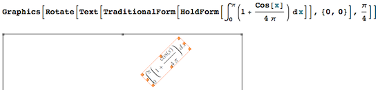
The annotated picture can be copied as PDF (I found I
have to select the bar on the right of the graphic first),
and pasted into other applications (e.g., Preview).
Likewise, the selected picture can be saved to a PDF file
via Edit → Save Selection As.... With
that added drawing capability, Mathematica makes it much
easier to create plots that don't require post-processing
in other applications such as Adobe Illustrator. You can
now go from Mathematica to your LaTeX document, or another
document preparation system, without detour.
However, use manual annotations with care: If you generated a plot programmatically and annotate it manually, then you will lose your manual edits when you later decide to change the programmatic part. Let's say you have a plot containing two curves, and manually added text to one of the curves. Later on, you decide to change the plot parameters of the other curve so you re-plot the graphic. Mathematica fortunately keeps your earlier annotated graphic in a separate Notebook cell, but the re-evaluated plot will of course have none of your manual annotations. So you have to proceed as in any other graphics editor: click to select your annotation in the original picture, and copy it. Then double-click back on the new plot to get a grey border around it, and do a paste. You should now have the old annotation in the new plot, at the correct relative position.
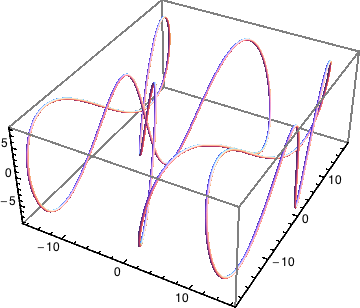
 When it
comes to manipulating graphics, one should distinguish
between annotations (adding content to
the picture), and edits (in the sense
of actually modifying the pictorial content). In
Mathematica, you can do both. In the
screenshot to the right, the spikes are not a
malfunction, they were edited in by hand. What you do
to edit a plot like this, is to double-click on the
graphic, then double-click on the curve. This makes the
individual points of the curve editable. The mouse can now
be used to drag them around. In
When it
comes to manipulating graphics, one should distinguish
between annotations (adding content to
the picture), and edits (in the sense
of actually modifying the pictorial content). In
Mathematica, you can do both. In the
screenshot to the right, the spikes are not a
malfunction, they were edited in by hand. What you do
to edit a plot like this, is to double-click on the
graphic, then double-click on the curve. This makes the
individual points of the curve editable. The mouse can now
be used to drag them around. In MMA version ≤ 8, you cannot directly
select the axis and tick labels and edit. However, MMA 8 lets you edit these labels to a certain extent after you outline all fonts as described below.
The same warning applies here as above: manual edits are "fragile", they get shoved aside when you re-evaluate your notebook cells. Use this with care!
On OS X, there are some nice PDF viewer applications such as Preview or Skim. In some cases you may find yourself copying PDF selections from one of those viewers directly into Mathematica, perhaps as part of a Mathematica-based presentation. This involvles selecting a rectangle in the original PDF file, copying to the system clipboard, and then pasting into a Notebook. However, when pasting from Preview into Mathematica 7.0.1 the rectangle that you origionally selected is ignored, and instead Mathematica displays the whole page from which the selection was taken. The fix for this is a script that can be found here. Some discussion of the issue took place on the Mathematica users mailing list.
In MMA version 8, this problem no longer
occurs, so my workaround script isn't needed here. However, there's a new bug:
PDF that has been copied and pasted from external applications will look jagged in the Notebook
when the view magnification is not 100%, and the PDF cannot be exported again. While this bug
isn't fixed, you may want to try the work-around on this page.
Copying graphical output from Mathematica to
Illustrator, the main issue concerns the fonts
and how to preserve them. This is dealt with below.
Another problem that occurs more sporadically is that
Illustrator may complain about your attempt to paste the
PDF: "Can't paste objects". This can happen
because Mathematica may have created invisible points in
your plot that are excessively far outside the plot
range.
 An example where
this occurs are parametric plots, as shown in this
Illustrator screen shot with everything selected, to reveal
points outside the plot region. In Illustrator
An example where
this occurs are parametric plots, as shown in this
Illustrator screen shot with everything selected, to reveal
points outside the plot region. In Illustrator
CS3, such plots can still be pasted by using
"Paste in front" instead of the general paste function.
However, this no longer appears to work in
CS4, so we'll need a different solution.
Specifying a PlotRange tells Mathematica only
which points are cropped from the displayed graphic (by the
"MediaBox", the black rectangle in the screen shot), but
these points are nonetheless present as hidden baggage in
the exported PDF. That's fine with most
PDF viewers, but not when pasting into
Illustrator. So how do you get rid of these unwanted parts
of the plot, if Illustrator doesn't let you paste? The
answer is to specify not only the
PlotRegion->{{xmin,xmax},{ymin,ymax}}, but
also RegionFunction -> Function[{x, y}, (xmin <
x < xmax) && (ymin < y < ymax).
This will force all the points outside the specified
rectangle to be dropped instead of just being
hidden from view.
The example plot here is properly truncated by the following code:
With[{xMin = -10, xMax = 10, yMin = -10, yMax = 10},
  ParametricPlot[Evaluate[Table[
     {u + Sin[u] Exp[-v], v - Cos[u] Exp[-v]},
     {u, -\[Pi], \[Pi], \[Pi]/10}]], {v, -10, 10}, Frame -> True,
   FrameLabel -> {"x", "y"},
   PlotRange -> {{xMin, xMax}, {yMin, yMax}},
   RegionFunction ->
    Function[{x, y}, (xMin < x < xMax) && (yMin < y < yMax)]]]
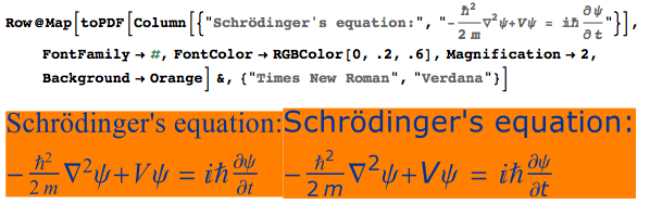
What if I want to copy a Mathematica formula as PDF, e.g., for a presentation? There is the menu item Edit → Copy As → PDF, which is often sufficient — this option inexplicably doesn't show up in the right-click context menu for a Notebook selection, so you have to go through the menu bar. However, you'll get a more customizable and predictable result using the following definition, which converts arbitrary Mathematica expressions (except images) to a vector drawing based on TraditionalForm:
toPDF[x_, opts : OptionsPattern[]] :=
  If[!ImageQ[x],
   First@ImportString[
     ExportString[
      Pane[Style[TraditionalForm[HoldForm[x]],
        FilterRules[{opts}, Options[Style]]],
       FilterRules[{opts}, ImageSize],
       BaseStyle -> {FontFamily -> "Times New Roman",
         Background -> (Background /. {opts} /. {Background ->
              None})}], "PDF"], "PDF", "TextMode" -> "Outlines"]
   ];
SetAttributes[toPDF, HoldFirst]
Now enter your formula as shown in this example:
toPDF[Integrate[1 + Sin[x]^2, {x, 0, Pi}], FontSize -> 18]
and you'll get a cropped graphics cell containing the PDF rendering (copying the formula from another cell works just as well, no matter what form it was in): ![]() .
.
The main features of this approach are:
PDF are outlined and hence will work in all external applications (see the related issue with Adobe Illustrator). TraditionalForm typesetting is hardcoded into the function.PDF.
To immediately copy the PDF to the clipboard, simply wrap the whole command in CopyToClipboard.
Here is another example showing different options for fonts, colors and magnification:
If the formula is too long, you can influence the line-wrapping by specifying the width w of the PDF using ImageSize -> w.
An alternative approach is to copy the formula expression as LaTeX, as described on a separate page.
But toPDF achieves almost the same thing without the intermediate step involving a LaTeX engine.
I find Mathematica's PlotLegends package unusable,
both for aesthetic and functional reasons.
So we'll have to craft our own legends. The challenge is how to
do this in a simple but flexible way that doesn't degenerate to a
completely manual process. By "manual," I mean to
hand-edit the legend using the drawing tools. That could be
a last resort — but here I'll explore alternatives.
The documentation for Inset, under "Applications,"
contains a custom legend construct of the form Epilog -> Inset[Panel[Grid[
...]]], and I'll try to improve on that.
In list plots with many data series, Mathematica provides great freedom of choice for the symbols identifying each series. The limits of this freedom are set by your imagination and by the bugs in ListPlot (see here for a version-7 bug that's been fixed in MMA 8.
In practice it may not be worth your time to try and
make up new plot markers. Since Graphics
accepts the Axes and Frame
options now, one can in principle make lower-level
constructs to create customized list plots, which however
forgoes the convenience of ListPlot options
such as DataRange.
If you let Mathematica make the choice for you with
PlotMarkers → Automatic, it generates a
reproducible but arbitrary combination of shapes and colors
for different sets of data in the same plot (i.e., when
plotting {dataSet1, dataSet2, ...}, you get a
unique plot marker style for each dataSeti).
In such plots, it is important to have a legend
that explains the meaning of the symbols.
As a prerequisite to making your own customized legends for a
ListPlot you need the list of plot
symbols and colors that Mathematica uses by default, so you
can tabulate them in your legend. This information isn't
easily extracted from the plot itself because it's
converted into graphics commands, so functions like
AbsoluteOptions don't reveal it. There is an undocumented function
Graphics`PlotMarkers[] that provides the sequence of plot symbols,
and the color information is available separately through
ColorData[1]; but I don't like Graphics`PlotMarkers[]
because it's syntax-colored as if it were an undefined variable. As a
solution, I devised the following function:
markerSymbols[n_] :=
 Drop[Drop[
    ListPlot[Transpose[{Range[n]}], PlotMarkers -> Automatic][[1, 2]][[1]],
     -1] /. Inset[x_, i__] :> x, None, -1]
It takes an integer argument n which is the number of
different plot markers you're using. The output is a list
with n entries representing the successive plot markers
from 1 to n. Each entry contains a list made up of the
color information and the symbol. The list format of the
output allows you to call this function once and store all
the plot markers for later use. If you just want to know,
e.g., what the 4-th plot marker looks like, the syntax
would be markerSymbols[4][[4]].
As an application of the markerSymbols function above,
let's now make a plot legend. Using Epilog -> Inset[Panel[Grid[...]]]
produces a result that looks nice on screen, but its smooth, rounded appearance
is lost when you convert to PDF/EPS.
The default style for Panel also causes fonts to be different from
the rest of the plot, so it could be better to replace Panel by Pane.
It is also possible to get a rounded appearance for our legend inset by means of
Framed[]. To proceed, it's useful to define the following function, which takes a set of text labels as its argument. Options you can specify include: the PlotStyle directives (i.e., color), the marker symbols (provided by markerSymbols, together with the colors), and the options accepted by Frame:
Options[legendMaker] =
  Join[FilterRules[Options[Framed],
    Except[{ImageSize, FrameStyle, Background, RoundingRadius,
      ImageMargins}]], {FrameStyle -> None,
    Background -> Directive[Opacity[.7], LightGray],
    RoundingRadius -> 10, ImageMargins -> 0, PlotStyle -> Automatic,
    PlotMarkers -> None, "LegendLineWidth" -> 35,
    "LegendLineAspectRatio" -> .2, "LegendMarkerSize" -> 8,
    "LegendGridOptions" -> {Alignment -> Left, Spacings -> {.4, .1}}}];

legendMaker[textLabels_, opts : OptionsPattern[]] :=
  Module[{f, lineDirectives, markerSymbols, n = Length[textLabels],
    x}, lineDirectives = ((PlotStyle /. {opts}) /.
       PlotStyle | Automatic :> Map[ColorData[1], Range[n]]) /.
     None -> {None};
   markerSymbols =
    Replace[((PlotMarkers /. {opts}) /.
         Automatic :> (Drop[
              ListPlot[Transpose[{Range[n]}],
                 PlotMarkers -> Automatic][[1, 2]][[1]], -1] /.
             Inset[x_, i__] :> x)[[All, -1]]) /. {Graphics[gr__],
         sc_} :> Graphics[gr,
         ImageSize -> ("LegendMarkerSize" /. {opts} /.
             Options[legendMaker,
              "LegendMarkerSize"] /. {"LegendMarkerSize" -> 8})],
      PlotMarkers | None :>
       Map[Style["", Opacity[0]] &, textLabels]] /.
     None | {} -> Style["", Opacity[0]];
   lineDirectives = PadRight[lineDirectives, n, lineDirectives];
   markerSymbols = PadRight[markerSymbols, n, markerSymbols];
   f = Grid[
     MapThread[{Graphics[{#1 /. None -> {},
          If[#1 === {None} || (PlotStyle /. {opts}) === None, {},
           Line[{{-.1, 0}, {.1, 0}}]],
          Inset[#2, {0, 0}, Background -> None]},
         AspectRatio -> ("LegendLineAspectRatio" /. {opts} /.
             Options[legendMaker,
              "LegendLineAspectRatio"] /.
              {"LegendLineAspectRatio" -> .2}), ImageSize -> ("LegendLineWidth" /. {opts} /.
             Options[legendMaker,
              "LegendLineWidth"] /. {"LegendLineWidth" -> 35}),
         ImagePadding -> {{1, 1}, {0, 0}}],
        Text[#3, FormatType -> TraditionalForm]} &, {lineDirectives,
       markerSymbols, textLabels}],
     Sequence@
      Evaluate[("LegendGridOptions" /. {opts} /.
          Options[legendMaker,
           "LegendGridOptions"] /. {"LegendGridOptions" ->
           {Alignment -> Left, Spacings -> {.4, .1}}})]];
   Framed[f,
    FilterRules[{Sequence[opts, Options[legendMaker]]},
     FilterRules[Options[Framed], Except[ImageSize]]]]];
Next, create an example plot:
plotExample = ListPlot[Evaluate[Table[RandomInteger[3 i, 10] + 2 i, {i, 3}]],
PlotMarkers -> Automatic, Joined -> True]
Finally, combine the plot with a legend:
Overlay[{plotExample,
  legendMaker[{"August",
    "September", "October"}, PlotMarkers -> Automatic, Background -> LightOrange,
   RoundingRadius -> 10]}, Alignment -> {Right, Top}]
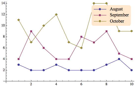
This procedure can be equally well applied to any other type of plot. The placement of the legend is controlled by the Overlay option Alignment -> {Right, Top}. Further discussion and examples of this function can be found in my post on StackExchange and a follow-up here. These links contain additional higher-level functions that can create legends "semi-automatically".
I decided to use overlays for legends because that makes it easier to place a single legend even when you're displaying several plots in a grid (see this post). A potential disadvantage is that the RoundingRadius is not referenced to the size of the actual plot, so you may have to adjust it manually after visual inspection. An overlay can't be mdified with the graphics editing tools in Matheamatica. That's why I defined a function deployLegend in the StackExchange post mentioned before, that flattens the legend into a graphics object combined with the plot. If you want to get a custom legend (from legendMaker) as a Graphics object that can be used in an Inset, the easiest way to do that is to use the function toPDF I defined above and insert toPDF@legendMaker[...].
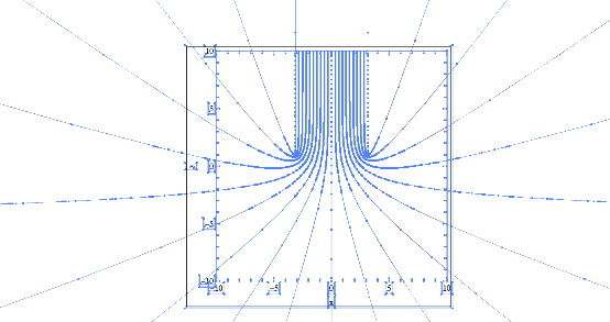
It is conventional in contour plots to label selected
contours by their height value. Often the labeling becomes
clearer if we also rotate that label so that it is
parallel to the corresponding contour. This alignment makes
the association between labels and contours easier to
discern, in particular when there are many contours close
together. Mathematica does not do this, and instead prints
all labels horizontally. The ContoutLabel
option allows you to customize labels but cannot be used to
rotate them. This is because the only information passed to
each label consists of the local coordinate and plot height
at the position of the label. For a rotation, you'd need to
know the direction of the contour through that point. Of
course we could get this information by calculating the
gradient of the function being plotted, but that will work
only with ContourPlot, and not with
ListContourPlot (which plots lists of points
instead of a function).
To at least partially solve this shortcoming, I wrote a
function rotateContourLabels which
post-processes Mathematica's contour plots to rotate all
included contour labels. The function assumes that you have
already made a contour plot with the option
ContourLabels->All or
ContourLabels->True. In the
post-processing, you can then specify an arbitrarily fancy
label style, which will be applied to the end result after
the necessary rotations have been calculated. This works
for ContourPlot and
ListContourPlot. As an example, let's go back
to the test plot in an earlier
ContourPlot issue,
im1 = ContourPlot[Im[(x + I y)^(1/2)], {x, -1, 1},
        {y, -1, 1}, Contours -> 20, ContourLabels ->
        True]
.
With the function as defined in the linked file contourPlotLabelsDescription.cdf, you can then invoke the following command to get the output shown on the right:
rotateContourLabels[im1, Text[#3, {#1, #2}, Background -> White] &]
The second argument is a function following the same
guidelines as in the Mathematica help for
ContourLabels.
The page linked here contains some custom density and contour plotting functions that produce more efficient graphics than the built-in Mathematica functions.
Mathematica's interactive drawing tools are only a meager subset of what a program like Adobe Illustrator can do, and so the interoperability between these two programs remains an important issue. I'll assume Illustrator CS 3 and Mathematica Version 6 here. If you're interested in older versions, check the web archive.
As you can tell from the archive link above, this page
has been online for many years, and for historical reasons
has been geared toward EPS as the main format.
With Mathematica V6, EPS format has ceased to
be the optimal vector format because it doesn't support
transparency or gradients well. So we should aim for
PDF export instead, in particular on a Mac
where this is the native graphics format.
The official
solution:
It turns out that we can completely fix all of
Illustrator's font problems with PDF and
EPS by executing the following cell
in Mathematica (assuming Mac OS X):
With[{temp = Directory[]},
If[ $Failed =!= SetDirectory["~/Library/Application\ Support/Adobe/Fonts/"],
 If[! MemberQ[FileNames[], "Mathematica"],
  CreateDirectory["Mathematica"];
  Run["/bin/ln -s " <> $InstallationDirectory <>
    "/SystemFiles/Fonts/Type1 " <> $HomeDirectory <>
    "/Library/Application\\ Support/Adobe/Fonts/Mathematica/"];
  SetDirectory["Mathematica"];
  Print[Style["Created symbolic link\n", Green], FileNames[],
   Style["\nin folder\n", Green], Directory[]],
  Print[Style[
    "Nothing to be done, folder already exists.\nTo re-install, first remove\n",
    Red], Directory[] <> "/Mathematica"]];
 SetDirectory[temp]]
]
This creates a new directory Mathematica in
the folder ~/Library/Application\
Support/Adobe/Fonts/, and places a symbolic link to
Mathematica's Type1 fonts in it. The symlink prescription
was sent to me by Aron Yoffe who got it from at Wolfram
Tech Support; I made it into a Mathematica script and added
an extra level to the directory structure to avoid
potential naming conflicts in Adobe's Fonts
folder.
If you prefer to install the fonts for multiple users,
replace ~/Library by /Library and
$HomeDirectory by $RootDirectory.
This cell only has to be re-evaluated if the Adobe
directory "/Library/Application Support/Adobe/Fonts/" is
modified (i.e., after updating Adobe products); but there
is no harm in repeating the instructions (the procedure
does nothing if the needed directory is already in
place).
Once you press shift-return on the above cell, you'll even be able to copy Mathematica graphics to the clipboard and paste it directly into Illustrator without the dreaded font substitution dialog. This is something that the two alternative methods below don't allow.
At this point it's worth pointing to a remark on another page
that also applies here: when exporting
annotated graphics from Illustrator, it's a good idea to
create outlines from fonts (Type > Create
Outlines) first.
Avoid font problems
by outlining text:
In Mathematica version 8, it is possible to implement within Mathematica my original approach of outlining all text in a graphic before exporting it. One advantage of doing this within Mathematica rather than in an external program is that you can ship the exported file directly to other users without worrying whether they have the necessary fonts installed.
To convert all text in a Graphics object gr to outlines (which are then filled curves and can be manipulated as such), type
outlinedGraphics = First@ImportString[ExportString[gr,"PDF"],"PDF","TextMode" -> "Outlines"]
The output can then be exported as PDF (or any other format) and will not contain any fonts that could trip up external programs. This approach works in MMA version 8. In version 7, the same approach produces buggy outlines in which separate glyphs are connected by extraneous lines.
Obsolete
solutions:
Below are my older workarounds for the Mathematica font
problem (in particular the first one still works fine). You
may want to explore these alternatives if you're not able
or willing to make the symbolic link as described above.
The potential advantage of these methods is that
they are more compatible with standard
installations, if you want to exchange graphics
files with other people.
Exporting from Mathematica to Illustrator works flawlessly if you make sure not to include special fonts in the exported file by setting the corresponding option as described below. To reiterate this point: you can use all the special fonts in your plot, but do not embed them in the exported EPS file so that Illustrator can instead look them up on its own among the Mathematica (and other) fonts it has available.
Export["test.eps",%, "EmbeddedFonts" ->
              False]
). This syntax is for Version 6. In
earlier versions, you would replace the option by
ConversionOptions -> {"IncludeSpecialFonts"
-> False}."EmbeddedFonts" option.| An example plot in Mathematica: | ⇒ | The result in Illustrator (from an earlier version): |
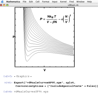 |
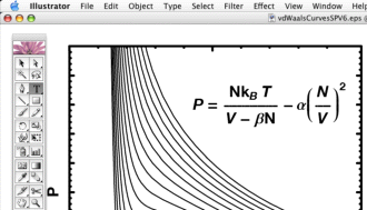 This is a random item from my thermodynamics
lecture, and the formula in the plot uses various
different fonts, including |
There are other programs that can convert EPS to PDF or other formats, and one can go through such a third program before importing into Illustrator. In particular, you can use ghostscript to strip away all fonts that cause trouble when importing into Illustrator, replacing them by outlines that are visually equivalent but can't subsequently be edited as text. Define the following Mathematica function:
epsExportNoFonts[exportName_, ob_] := Module[{},
    Export[exportName, ob, "EPS"];
    Run["gs -sDEVICE=epswrite -dNOCACHE -sOutputFile=nofont-" <>
        exportName <> " -q -dbatch -dNOPAUSE "  <> exportName <> " -c quit"]]
Then use this function instead of the
built-in Export[] to write your
Mathematica plot as an eps file:
epsExportNoFonts["myfile.eps", graphics].
This function writes two EPS files: one called
myfile.eps and a second one called
nofont-myfile.eps. The file with
nofont- prepended can be imported into
Illustrator and should cause no font substitution
problems. If Mathematica returns with a "0", there was
no error. If the return code is something else, it may
be because gs is not found. This could
mean that you don't have ghostscript installed, or that
you need to provide the path information, by replacing,
in the above code, Run["gs... with
Run["/sw/bin/gs (or whatever the path is
that you get from which gs in the
Terminal). On my system, this is not necessary because
I have a file .MacOSX/environment.plist
through which this path information is provided to
applications such as Mathematica.