Labels in Mathematica 3D plots

This is the HTML version of a Mathematica 8 notebook. You can copy and paste the following into a notebook as literal plain text. For the motivation and further discussion of this notebook, see "3D Text Labels" on the main Mathematica graphics page.

label3D

The function label3D takes an arbitrary expression and displays it as a textured 3D rectangle with transparent background. The expression is converted to an image without being evaluated. By default, regions matching the color at the corner of the image are made transparent. Alternatively, you can explicitly specify which color to make transparent by adding the option "TransparentColor" -> White to label3D (instead of White, the color can be anything you like).

label3D[s_, pos_, xVec_, tiltAngle_, opts : OptionsPattern[]] :=
 Module[{ra, width, height, r},
  ra = Rasterize[
        Style[HoldForm[s], FilterRules[{opts}, Options[Style]], Magnification -> 10], 
          Evaluate@Apply[Sequence, FilterRules[{opts}, Options[Rasterize]]], "Image"
       ];
  {width, height} = ImageDimensions[ra];
  r = SetAlphaChannel[ra, With[
     {
      color = Apply[List, 
        ColorConvert[
         "TransparentColor" /. {opts} /. {"TransparentColor" -> 
           Apply[RGBColor, ImageData[ra][[2, 2]]]}, "RGB"]
       ]
      }, Binarize[ra, (Norm[# - color] > .005)&]]
   ];
  Translate[(* // to make lefthand corner pos *)
   Rotate[(*   // around z axis *)
    Rotate[ (* // around y axis *)
     Rotate[(* // tilt around x axis *)
      Scale[ (*// to make width equal |xVec| *)
       {EdgeForm[FrameStyle /. {opts} /. FrameStyle -> None],
        Texture[ImageData@r],
        (* // Texture fills polygon initially in the xz plane *)
        Polygon[{{0, 0, 0}, {width, 0, 0}, {width, 0, height}, {0, 0, height}}, 
         VertexTextureCoordinates -> {{0, 0}, {1, 0}, {1, 1}, {0, 1}}]},
       Norm[xVec]/width, {0, 0, 0}
       ],
      tiltAngle, {1, 0, 0}],(* // x rotation *)
     Arg[Chop@N[Norm[xVec[[1 ;; 2]]] + I xVec[[3]]]], {0, -1, 0}], (* // y rotation *)
    Arg[Chop@N[xVec[[1]] + I xVec[[2]]]], {0, 0, 1}
   ], (* // z rotation *)
   pos]
  ];
SetAttributes[label3D, HoldFirst]

Example and explanations

1. The first argument is the object to be displayed.
2. The second argument is the position of the bottom left corner of the label.
3. The third argument is a vector pointing in the direction along which the baseline of the label should be oriented. The length of this vector is taken as the width of the the label.
4. The fourth argument is the angle (in radians) by which the label is rotated around its baseline.
5. The options Magnification (and also ImageSize) determine the resolution of the rasterized label, and also influence the line breaking in wide labels. Without the option FrameStyle, there will be no frame around the label.

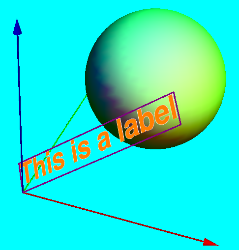
Here is a simple example showing the relation to the coordinate axes:

With[{position = {0,0,0}, direction = {1.5, 0, 1.3}, tiltAngle = -.8},
 Graphics3D[
 {
  {Green, Specularity[2], Sphere[{1, 1, 1}, .7]},
  Map[{Apply[RGBColor, #], Arrow[Tube[{{0, 0, 0}, #}]]} &, 
        2 IdentityMatrix[3]
     ],
  {Glow[White],
    label3D["This is a label", 
            position, direction, tiltAngle, 
            FontColor -> Orange, FontSize -> 18, 
            FontFamily -> "Helvetica", 
            FontWeight -> Bold, Magnification -> 4,
            FrameStyle -> Directive[Purple, Thick]
           ]
  }
 }, 
 Boxed -> False, SphericalRegion -> True, Background -> Cyan
 ]
]
    

Note in particular the additional Glow[White] which makes the appearance of the labels independent of the light sources in the plot. I think that's a good way to set your labels apart from the rest of the plot.

Going wild

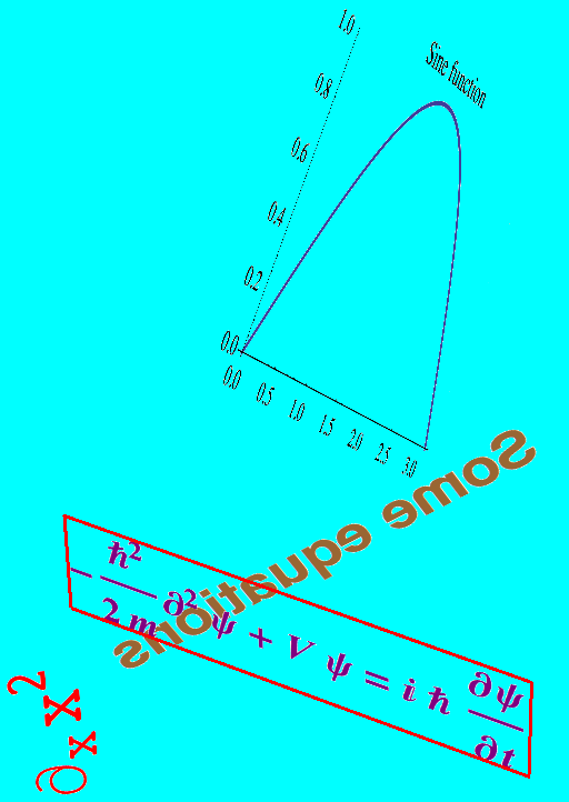
The following shows several different ways to use this function, combined in one graphic. The example also illustrates different ways of providing style options.

Graphics3D[
{
 Glow[White], 
  label3D[
    \!\(\*SubscriptBox[\(\[PartialD]\), \(x\)]\*SuperscriptBox[\(x\), \(2\)]\), 
    {0, -.6, 0}, {0, 0, 0.5}, π/4, 
    FontColor -> Red
  ], 
  label3D[Evaluate@
    Plot[Sin[x], {x, 0, \[Pi]}, PlotLabel -> "Sine function", 
     BaseStyle -> {FontSize -> 6}], 
    {0, 0, 1}, {0, 1.2, -1.2}, 0
  ], 
  label3D[Evaluate@
    Style[TraditionalForm[
      "-\!\(\*FractionBox[SuperscriptBox[\(\[HBar]\), \(2\)], \(2  \
      m\)]\)\!\(\*FormBox[SuperscriptBox[\(\[PartialD]\), \(2\)],
TraditionalForm]\) \[Psi] + \!\(\*
      StyleBox[\"V\",\nFontSlant\
->\"Italic\"]\) \[Psi] = \[ImaginaryI] \[HBar] \!\(\*FractionBox[\(\[PartialD]\[Psi]\), \
      \(\[PartialD]t\)]\)"
         ], 
        Purple, Bold
    ], 
    {-.5, 0, 0}, {1.5, 0, 0}, 0, 
    FontFamily -> "Times New Roman", Magnification -> 5, 
    FrameStyle -> Directive[Thick, Red]
  ],
  label3D[
    "Some equations", 
    {.7, .7, .5}, {-1, -.7, -.7}, 0, 
    FontColor -> Brown, FontSize -> 14, FontFamily -> "Helvetica", 
    FontWeight -> Bold, Magnification -> 5
  ]
}, Boxed -> False, SphericalRegion -> True, ImageSize -> 500,
Background -> Cyan
]

Above, I have to use Evaluate explicitly when the argument is not supposed to be taken literally, as in the sine function plot and in the framed equation with additional styles applied.