Non-orthogonal
Designs & Unequal N's
I. The
problem
A.
Missing data causes the partial confounding of effects of independent
variables.
B. Can occur
in both experimental and observational designs.
C.
Can be due either to design or happenstance.
1. Subjects
may fail to respond, die, disappear, etc.
The result is unequal N's.
Analysis of experiments with missing data will depend on the source of
the missing data. If the missing data
is not due to random processes (e.g. equipment failure), then the validity of
the study is in doubt (e.g. depressives may not have enough energy to come in;
agoraphobics may not go out). If the
data are apparently missing at random then one can proceed as described below.
2.
Experimenters may intentionally omit some conditions. In observational research, some combinations
of factors rarely occur; e.g., whites rarely kill blacks. If one over-samples cells with small
population N's to achieve equal sample N's, then one cannot make reasonable
statements about the larger population without correcting for sample selection
biases.
II.
Data Missing by Experimental Design
A. Fractional Designs: Several classic experimental designs have
partial confounding of independent variable effects. We will consider only one: Latin Square.
B. Latin Square (many
possible squares).
1. Example
A(3) X B(3) X C(3) Latin Square
A
B
1 2 3
1 C1 C2 C3
2 C2 C3 C1
3 C3 C1 C2
If this were a completely crossed design would have:
A
B C 1 2 3
1 1 X
2 X
3 X
2 1 X
2 X
3 X
3 1 X
2 X
3 X
Instead, have only the cells marked with X's. This causes the interactions to be
confounded with the main effects:
a) Linear model for this Latin Square (variables
representing factors A, B, and C grouped inside brackets):
Y=
a +{b1A1 + b2A2}+ {b3B3
+ b4B4}+{b5C5+b6C6}+e
b) Linear model for the corresponding completely crossed design:
Y= a +{b1A1 + b2A2}+
{b3B3 + b4B4} + {b5C5+b6C6}
+ {b7A1B3+b8A1B4+b9A2B3+b10A2B4}
+ {b11A1C5+b12A1C6+b13A2C5+b14A2C6} + {b15B3C5+b16B3C6+b17B4C5+b18B4C6}
+ {b19A1B3C5...}+e
c) The standard analysis of a Latin square design rests on the assumption that the interactions between the independent variables are non-existent.
Source df E(MS)
A p-1 nps2a + s2s(abc)
B p-1 nps2b + s2s(abc)
C p-1 nps2c
+ s2s(abc)
Residual (p-1)(p-2) s2res + s2s(abc)
Within
cell p2(n-1) s2s(abc)
p=number of levels of factors. Residual is
"interaction" term. In a
completely crossed design, would have:
Source df E(MS)
A a-1 nbcs2a + s2s(abc)
B b-1 nacs2b + s2s(abc)
C c-1 nabs2c + s2s(abc)
AB a-1(b-1) ncs2ab + s2s(abc) ------------
AC a-1(c-1) nbs2ac + s2s(abc) Latin Square
BC b-1(c-1) nas2bc + s2s(abc) assumes = 0
ABC a-1(b-1)(c-1) ns2abc + s2s(abc) ------------
S(ABC) abc(n-1) s2s(abc)
Therefore, a partial test of the appropriateness of
a classic Latin square analysis is to test the "Residual" MS against
the within-cell MS (i.e. F=MSres/MSwithin).
This is not a reliable test because if interactions exist, some of their
effect will be attributed to the main effects with which they are correlated.
2. Example (Winer, p. 698): 3 hospitals (A), 3 drugs (B), and 3 types of
patients (C)
Design Data
B B
A
1 2 3 1 2
3
1 C2 C3 C1
2 5 3 1 9
10 12 12 2 2 4 6
2 C3 C1 C2
6 8 12 7 0 2 2 5 0 0 1 4
3 C1 C2 C3
0 1 1 4 0 1
1 4 2 1 1 5
Means
B
A 1 2
3
C1=2.42 1 2.75 10.75 3.50 5.67
C2=1.83 2 8.25 2.25 1.25 3.92
C3=7.08 3 1.5 1.5 2.25 1.75
4.17 4.83 2.33
![]()
![]()
![]()
![]()
![]()
SSresidual=SSbetween
cells-SSA-SSB-SSC= 33.39
|
Source |
SS
|
df |
MS |
F |
|
|
|
|
|
|
|
A |
92.39 |
2 |
46.20 |
12.52* |
|
B |
40.22 |
2 |
20.11 |
5.45* |
|
C |
198.72 |
2 |
99.36 |
26.93* |
|
Residual |
33.39 |
2 |
16.70 |
4.53* |
|
Within |
99.50 |
27 |
3.69 |
|
Note: the significant residual effect suggests that
a Latin Square analysis is inappropriate.
III. Dealing with Sporadic Missing data
A. Drop
variables: One may exclude
variables when a substantial proportion of the cases do not have data on that
variable. This may lead to
misspecification (omitted variable) error.
B. Drop
subjects: One may eliminate
subjects from the analyses ("list wise deletion") if the proportion
of subjects with missing data relative to the total N is small and the data are
missing at random. This will not
seriously affect the results, except to decrease the statistical power of the
other estimates. If the data are not
missing at random, then this procedure may lead to biased estimates.
C. Regression
on the missing data correlation matrix.
Correlations between pairs of independent variables may be calculated
after deleting cases on which information on either one of the variables is
unavailable. In the extreme case, this
may cause the correlations in the matrix to be based on separate subsets of the
data and the resulting correlation matrix may violate the mathematics of
correlation matrices; i.e., it may be impossible to obtain some of the
correlations in the matrix with a set of complete data.
1. For example, r12
is mathematically constrained to lie within the range defined by:
![]()
Only when r13=0
or r23=0 can the value of r12 range between -1 and +1.
2. For
example, in the matrix below r12, r13, and r23
would be calculated using entirely different sub-samples.
S Y X1 X2 X3
1 1 . 2 4
2 2 . 3 5
3 4 2 . 5
4 2 2 . 3
5 2 3 4 .
6 3 5 2 .
D. Create missing value variable.
1. Qualitative variables:
a. Add a
“missing” category
b. For example,
race may be coded as white, black, Hispanic, Asian, or other. This would be coded as k-1=4 dummy
variables. Missing values could be
coded as another category, e.g. white, black, Hispanic, Asian, other, or
missing. This would appear as k-1=5
dummy variables which would be interpreted as usual.
2. Quantitative
variables:
a. Create a new variable (the missing value indicator) that indicates whether the data on the predictor is present. Then replace missing values with a constant. Together, these two variables (the missing value indicator and the predictor with missing values plugged by a constant) contain all of the information needed. In multiple regression, these variables must be treated as a set and always entered or deleted together.
b. Regress the missing value indicator variable on the
criterion. Then add the variable with
the missing values. The b for the
indicator variable is meaningless, but the b for the original variable is the
slope of the regression line for the cases with the values present. The intercept is also the intercept for the
cases with data present.
c. If the missing values are plugged with the variable mean, then a
non-hierarchical regression may be used since then the missing value indicator
and the original variable are uncorrelated.
d. For example, let X1=0 when data on X2 are present; let X1=1 when
data on X2 are absent. Then regress Y =
a +b1X1 + b2X2. When data on X2 are present, this will yield
the equation: Y = a + b2X2
e. Note: Plugging missing
values with the variable mean without creating a missing value indicator will
artificially increase the N and decrease the variance.
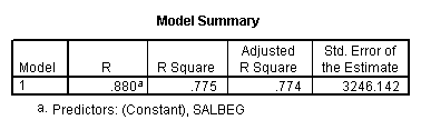
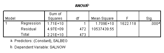
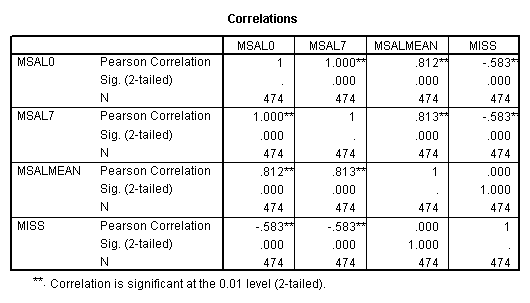
E. Example
Regression on full data.

Regression on data with several observations missing.
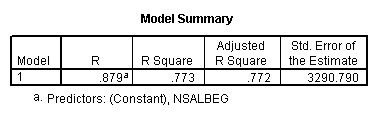

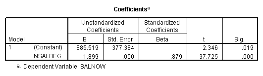
Regression on data with missing value indicator and missing values replaced by mean.
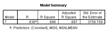
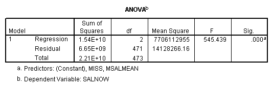
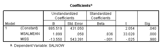
Regression on data with missing value indicator and missing values replaced by 0.


Regression on missing value indicator and missing data replaced by 7.
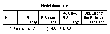
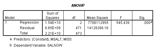
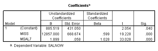
Note that when the missing values are plugged by the mean, the missing value indicator is not correlated with this variable. If the missing values are plugged by other numbers, the missing value indicator will be correlated with this variable and the value and significance of the coefficient for the missing value indicator will be altered.
IV. Types
of Sums of Squares and Mean Squares
1. To test
MS for an effect one must partition the SS.
When the correlation between the independent variables equals zero,
there is no problem. When the
correlation is non-zero, then there are several possible strategies:
a. Type I SS: SS for variable is equal to the increment in the SS explained by
the model as each variable is added.
This is useful if there is a theoretical ordering for the variables,
otherwise the estimates of the effects of variables placed in the model early
will be contaminated by the effects of variables left out of the model at that
stage.
b. Type II
SS: SS for each variable is equal to the
increment in the SS explained by the model when that variable is added to the
model after all other main effects.
This is useful to test the hypothesis that a variable has no
"unique" effect.
c. Type III: SS is determined from the result of a "contrast"
analysis using weights so that the estimates of the individual effects are not
biased by the pattern of cells present in the model. This is essentially an artificial "orthogonalization"
of the effects.
1.
An
entire analysis or an hypothesis test can be performed using orthogonal
coding. When orthogonal contrasts are
created using the standard procedure, the sum of the contrast weights must
equal zero. When there are unequal n’s,
predictors coded using these weights will be correlated and the tests performed
on them will reflect tests of unweighted means.
2.
If
contrast codes are developed so that:
L=n1c1+n2c2+...nkck=0,
then predictors coded using these weights will be uncorrelated and the tests
performed on them will reflect tests of weighted means.
d. When the
independent variables are uncorrelated, all of these methods will yield
identical effects. Note: bj's
are always interpretable -- providing the problems of correlations between the
independent variables are recognized.