Tomographic Imaging Environment for

Ridge Research and Analysis

TIERRA

Developed by: Andrew Barclay, Robert Dunn and Douglas Toomey University of Oregon, Eugene, OR 97403

TIERRA was developed to allow tomographic imaging of seismic structure using travel time data from active source experiments. The tomography code is written in Fortran 77. Much of the I/O and plotting of results is done using Matlab 5.

Descriptions of the tomographic method may be found in the following papers:

Toomey, D. R., S. C. Solomon and G. M. Purdy, Tomographic imaging of the shallow crustal structure of the East Pacific Rise at 9 30'N, J. Geophys. Res., 99, 24,135-24,157, 1994.
Dunn, R. A. and D. R. Toomey, Seismological evidence for three-dimensional melt migration beneath the East Pacific Rise, Nature, 338, 259-262, 1997.
Barclay, A. H., D. R. Toomey, G. M. Purdy, and S. C. Solomon, Seismic structure and magmatic accretionary processes at the Mid-Atlantic Ridge, 35N, J. Geophys. Res, 103, 17,827-17,844, 1998.

Control parameters
Station locations
Velocity model
Carving model (not implemented)
Travel time data
Gridded bathymetry
Perturbational model: Isotropic velocity
Perturbational model: Anisotropic velocity

Coordinate Systems
Output Files
Structure of the program

Installing TIERRA

Obtain the tar file
Untar
Read the README file
An example Makefile is included.

Input Files

Control parameters

The control file is used to set parameters for a run. Parameter names and definitions are given below.

**CONTROL FILE PARAMETERS**
nsts	Number of stations
nsht	Number of shots
npdsc	Number of pick descriptions (data types)
pick	Array of pick descriptions
nitmax	Maximum number of forward and inverse iterations
lsqr_its	Number of least squares iterations
q_du_p	Lagragian multiplier on isotropic model length
q_du_sxy	Lagrangian multiplier for horizontal isotropic smoothing
q_du_sz	Lagrangian multiplier for vertical isotropic smoothing
q_da_p	Lagrangian multiplier on norm of percent anisotropy model
q_dt_p	Lagrangian multiplier on norm of azimuthal anisotropy model
q_da_sxy	Lagrangian multiplier for horizontal anisotropic smoothing
q_da_sz	Lagrangian multiplier for vertical anisotropic smoothing
xhalf_a	Anisotropy smoothing length, x direction
yhalf_a	Anisotropy smoothing length, y direction
zhalf_a	Anisotropy smoothing length, z direction
tf_in_tt	Logical: Read in TT files on first iteration?
tf_out_tt	Logical: Write out TT files after first iteration?
tf_syn_tt	Logical: Write out synthetic data for the starting model?
tf_out_dws	Logical: Write out derivative weight sum?
tf_out_A	Logical: Write out the sparse A matrix?
tf_line_integrate	Logical: Perform Line Integration during ray tracing?
tf_carve	Logical: Carve out sections of the slowness model for faster ray tracing?

Example ascii file: control.test*

7 863 1 nsts, nsht, npdsc

1 picktypes to use

4 100 nitmax, lsqr_its

1. q_du_p = 1 won't mess uncertainties

100,100 q_du_sxy, q_du_sz

1., 1. q_da_p, q_dt_p = 1 won't mess uncertainties

100,100 q_da_sxy, q_da_sz

1.1,1.1,1.1 xhalf_a, yhalf_a, zhalf_a

f,f tf_in_tt, tf_out_tt

f,f tf_syn_tt, tf_out_dws

f,f tf_out_A, tf_line_integrate

f tf_carve

* The control file is an unformatted ascii file. The only restriction is that each line of the file must be organized as above. The variable names and comments to the right are not read in.

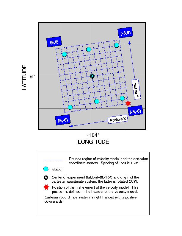
Station locations

The station file inputs the location of the stations and the center of the coordinate system. Station locations are defined by latitude and longitude. The table below shows the variable definitions.

**DEFINITION OF PARAMETERS IN A STATION FILE**
ltdo	Latitude of coordinate center (degrees only, postivie to north)
oltm	Latitude of coordinate center (decimal minutes)
lndo	Longitude of coordinate center (degrees only, +'ve to east)
olnm	Longitude of coordinate center (decimal minutes)
rota	Rotation of cartesian coordinate system in degrees (+'ve is CCW)
zdatum	Mean depth of seismic array relative to sea level (kilometers)
istn(nsta)	Station number (integer)
ltds(nsta)	Latitude of station (degrees only, postive to north)
sltm(nsta)	Latitude of station (decimal minutes)
lnds(nsta)	Longitude of station (degrees only, positive to east)
slnm(nsta)	Longitude of station (decimal minutes)
ielev(nsta)	Depth of instrument (meters)

Example ascii file: station.dat*

9 31.740 -104 14.656 8 2.882

7

3 9 31.740 -104 14.656 2579

4 9 26.765 -104 18.940 2888

5 9 27.433 -104 14.169 2595

6 9 28.087 -104 9.259 2893

15 9 36.721 -104 10.529 2901

31 9 36.028 -104 15.495 2563

33 9 35.126 -104 19.705 2895

*The station file is an unformatted ascii file. Defintions of each line of the file are as follows:

**VARIABLES IN STATION FILE BY LINE**
Line 1	ltdo, oltm, lndo, olnm, rota, zdatum
Line 2	nsta (number of stations to be read in)
Line 3:nsta	istn(i), ltds(i), sltm(i), lnds(i), slnm(i), ielev(i)

Velocity model

Carving model

Travel time data

The event file inputs the source parameters and travel time observations for each station.

**DEFINITION OF PARAMETERS IN A EVENT FILE**
nshot(nsht)	Shot number
iyr(nsht)	Year of event
imo(nsht)	Month of event
iday(nsht)	Day of event
ihr(nsht)	Hour of event
mino(nsht)	Minute of event
seco(nsht)	Second of event
ltde(nsht)	Event latitude (degrees, integer)
eltm(nsht)	Event latitude (decimal minutes)
lnde(nsht)	Event longitude (degrees, integer)
elnm(nsht)	Event longitude (decimal minutes)
dep	Event depth (km beneath sea-level for shots)
ista(nsts)	Station indentifier (integer)
ides(nsts)	Pick description (e.g., 1)
sdev(nsts)	1 sigma uncertainty in travel time (sec)
secp(nsts)	P wave travel time (sec)

Example ascii file:

2123 971120 054 12.404 9 49.709 -104 6.158 0.01

2 5 16 20 23 25 27 50 51 52 53 54

0 0 0 0 0 0 0 0 0 0 0 0

0.023 0.000 0.000 0.015 0.000 0.000 0.015 0.000 0.015 0.000 0.000 0.000

8.730 0.000 0.000 8.219 0.000 0.000 8.172 0.000 9.857 0.000 0.000 0.000

2124 971120 057 42.275 9 49.467 -104 6.124 0.01

2 5 16 20 23 25 27 50 51 52 53 54

0 0 0 0 0 0 0 0 0 0 0 0

0.023 0.000 0.000 0.015 0.000 0.000 0.015 0.000 0.015 0.000 0.000 0.000

8.697 0.000 0.000 8.200 0.000 0.000 8.178 0.000 9.807 0.000 0.000 0.000

**VARIABLES IN EVENT FILE BY LINE**
Line 1	nshot, iyr, imo, iday, ihr, mino, seco, ltde, eltm, lnde, elnm, dep
Line 2	ista(nsts)
Line 3	ides(nsts)
Line 4	sdev(nsts)
Line 5	secp(nsts)
Line 6	Blank line (also at very end of file).

As of November 3, 1998 the first line of the event file is (unfortunately) formatted. The format
is as follows:

READ(4,4001,END=9999) nshot(n),iyr(n),imo(n),iday(n),

& ihr(n),mino(n),seco(n),

& ltde(n),eltm(n),lnde(n),elnm(n),dep

4001 FORMAT(i4,1x,i2,i2,i2,1x,i2,i2,1x,f6.3,i4,1x,f6.3,1x,i4,1x,f6.3,f7.2)

Gridded bathymetry

The bathymetry file is used to map the velocity model graph to the seafloor. The file is an
unformatted binary file (as of Nov. 3, 1998).

Notes on the bathymetry file:

Bathymetry must be defined on a regular grid, typical grid spacing of 100 to 150 m.
The bathymetry map must circumscribe the velocity model and thus the positions of all sources and receivers.
The variables (rlatmin,rlongmin) and (rlatmax,rlongmax) define the lower-lefthand and upper right-hand corners of the map.

**VARIABLES IN BATHYMETRY FILE**
rlongmin	Minimum longitude of map area (decimal degrees; north and east of Greenwich are positive)
rlongmax	Maximum longitude of map area.
rlatmin	Minimimum latitude of map area.
rlatmax	Maximum latitude of map area.
gsmin	Grid interval in decimal minutes.
ncol_cb	Number of columns in the map.
nrow_cb	Number of rows in the map.
z_cb(i,j)	Depth in meters; positive below sea-level.

Here is how to make a binary map:

First, it is presumed that you have used GMT to make and gridded file which is stored in NetCDF format.
Run grd2xyz to output an ascii file of triplets.
Reformat this ascii file using something like the fortran program reformat_bathy.f

Perturbational model: Isotropic velocity

Perturbational model: Anisotropic velocity

Coordinate Systems

Their are several coordinate systems used. Sit down, have a cup of tea and carefully read the following:

Geographical Coordinate System (GCS): Defined by latitude and longitude. North and east of Greenwich are positive. The following use this coordinate system:

Station locations as defined in the station file (blue circles in figure).
Source locations as defined in the event file (not shown in figure).
The bathymetric map. It's origin is in the lower left hand corner of the study area (shown by grey region in figure).

Cartesian Coordinate System (CCS): Defined by x and y positions. The CCS is right-handed with z positive downwards (see figure). The position of the CCS is defined in the header of the velocity model (in the figure below the red sun indicates the origin of the CCS). Within the TIERRA, all real work is done in this system (i.e., geographical positions are converted to cartesian coordinates before ray tracing or inversion). The following use this coordinate system:

Velocity model (surface of velocity model is indicated by blue mesh in figure).
Perturbational models (not shown in figure).

Important Notes:

The bathymetric map MUST circumscribe the cartesian coordinate system.
The velocity model, which coincides with the CCS, MUST circumscribe all source and receiver positions.
For 3-D models, the spatial limits of the perturbational model must be equal to the spatial limits of the velocity model. Perturbational models can be 1- or 2-D, provided that the limits of the ordinates with perturbational nodes equal the limits of the velocity model.

forward model
perturbation model
coordinate systems

Output Files

Structure of the program

Begin

Load Input Files

Input control parameters
Input station list, set up coordinates
Input Velocity (slowness) and anisotropy model
Input Carving File
Input travel time data
Input in the traveltime set logical file
Input the SEABEAM data
Input slowness perturbation model
Map from Graph1 (vel. grid) to Graph3 ( perturb. grid)
Input anisotropy perturbation model (anis (r,t,p))
Map from Graph1 to Graph3 anisotropy
Hang Slowness grid from the Sea Beam map
Read in the Arc Set for ray tracing
Open a file for the travel time residuals and other information

Start Main Loop over forward and inverse problem iterations

Forward Problem

Loop over stations and events
calculate the TT fields,
calculate residuals
calculate medium derivatives, load A matrix

Inverse Problem

Apply a priori covariance constraints
Calculate the solution
Write solution to disk

End Main Loop
Output synthetic travel time data if desired

END

Input Routines & Files

SUBROUTINE inputStations

! Reads in the station list, sets up the coordinate system,
! and calculates the stations' cartesian coordinates.
!
! Zdatum: Reference depth within array. For a flat model it is the
! depth of the seafloor
!
! Subroutines required: setorg; disto;

! common block variables:
      INCLUDE 'Params.f'
      INCLUDE 'Contrl.f'
      INCLUDE 'Observ.f'
      INCLUDE 'Shortd.f'
      INCLUDE 'Zdatum.f'

! Variables Read

! Store station coordinates
         station(1,j)=x
         station(2,j)=y
         station(3,j)=z

SUBROUTINE inputVelmodel

! This routine reads in the velocity model in the
! form of velocity specified on a graph. The nodal spacing
! is constant for a given (x,y,z)-ordinate.
!
! The header has 12 elements
!       glnkm      - Dist. in long.-dir. to graph origin wrt Coord. Cen.
!       gltkm      - Dist. in lat.-dir. to graph origin wrt Coord. Cen.
!       rlong(min) - N/A
!       rlong(max) - N/A
!       rlat(min) - N/A
!       rlat(max) - N/A
!       nx         - Columns of data
!       ny         - Rows of data
!       nz         - Planes of data
!       gx         - X interval (km)
!       gy         - Y interval (km)
!       gz         - Z interval (km)
!       matrix of gridded data is written:
!               do k=1,nz
!                  do j=1,ny
!                     write(1)(vel(i,j,k),i=1,nx)
!                  end do
!               end do

! common block variables:
     INCLUDE 'Params.f'
      INCLUDE 'Contrl.f'
      INCLUDE 'Graph1.f'
      INCLUDE 'Graph2.f'
      INCLUDE 'Graph7.f'
      INCLUDE 'MatLab.f'

SUBROUTINE inputCarve

! Reads Matlab file of carved region for each reciever
! and its pick types (Up to 5 pick types and 5 regions
! for each pick type.)
!
! Format of Mat file:
!
! carve = [station# #ofpicktypes #ofregionsforptype1 #ofregionsforptype2 ...
! xmin xmax ymin ymax zmin zmax xmin xmax ...]

! common block variables:
      INCLUDE 'Params.f'
      INCLUDE 'Contrl.f'
      INCLUDE 'MatLab.f'
      INCLUDE 'Intrvl.f'

! Variables read

carve

SUBROUTINE inputTT

! Reads in the P travel times for ALL stations in the station list.
! First source parameters are read, then station names, pick types,
! weights, and travel times.
!
! 1) All stations in the station file must report a
!    travel time; a zero time is used to indicate shots
!    without an observation.
!
! 2) An array sdev(nsta,nevt) has been added to record estimates
!          observational standard deviation in seconds.
!
! 3) An array ides(nsta,nevt) has been added to describe the
!    the arrival type (secondaries , P, PmP, Pn, etc..)
!
! Arrivals at stations not in the station list are discarded;

! Common block variables:
      INCLUDE 'Params.f'
      INCLUDE 'Contrl.f'
      INCLUDE 'Events.f'
      INCLUDE 'Observ.f'
      INCLUDE 'Stodat.f'

SUBROUTINE inputBathym

! Inputs Sea Beam data file.

! Common block variables:
      INCLUDE 'Params.f'
      INCLUDE 'Contrl.f'
      INCLUDE 'Observ.f'
      INCLUDE 'Bathym.f'
      INCLUDE 'Shortd.f'
      INCLUDE 'Zdatum.f'

SUBROUTINE inputUPertModel

! Reads in the parameterization for the pertubation model.
! Defined on a uniform but not necessarily evenly spaced set
! of grid points.
!
! The origin of the coordinate system is at (x,y,z)=(0,0,0)
! which will not in general correspond to the point
! xn(1),yn(1),zn(1).

! Common block variables:
      INCLUDE 'Params.f'
      INCLUDE 'Graph1.f'
      INCLUDE 'Graph2.f'
      INCLUDE 'Graph3.f'
      INCLUDE 'Contrl.f'

SUBROUTINE inputAPertModel

! Reads in the params for the anisotropy pertubation model.
! Defined on a uniform but not necessarily evenly spaced set
! of grid points.
!
! The origin of the coordinate system is at (x,y,z)=(0,0,0)
! which will not in general correspond to the point
! xn(1),yn(1),zn(1).

! Common block variables:
      INCLUDE 'Params.f'
      INCLUDE 'Graph1.f'
      INCLUDE 'Graph2.f'
      INCLUDE 'Graph8.f'
      INCLUDE 'Graph7.f'
      INCLUDE 'Contrl.f'

! Reads      READ(3,*) nxda,nyda,nzda
         READ(3,*) (xnda(i),i=1,nxda)
         READ(3,*) (ynda(j),j=1,nyda)
         READ(3,*) (znda(k),k=1,nzda)
         READ(3,*) dummy(k)

SUBROUTINE inputTTset

! This routine reads in the logical "inTTset" which
! states which reveivers and pick types require raytracing

! Common block variables:
      INCLUDE 'Params.f'
      INCLUDE 'Contrl.f'
      INCLUDE 'Observ.f'
      INCLUDE 'MatLab.f'

! Variables read in:

inTTset    ::    LOGICAL Matrix (ones and zeros)
                            Row number equals station number
                             Column number equals pick type

example:
0 0 0

SUBROUTINE inputArcSet

! Procedure to read and construct a forward star template

! Common block variables:
      INCLUDE 'Params.f'
      INCLUDE 'Graph2.f'
      INCLUDE 'ArcSet.f'
      INCLUDE 'Contrl.f'
      INCLUDE 'MatLab.f'

readTT

SUBROUTINE readTT(ns,ptype)

! This routine may be called iteratively.
! It inputs:
! > Travel times t(nodes$)
! > Ray paths iprec(nodes$)
!
! Format:
! > binormat_ray = true Binary unfomatted
! > binormat_ray = false Mat-file format.

! Common block variables:
      INCLUDE 'Params.f'
      INCLUDE 'Contrl.f'
      INCLUDE 'Graph1.f'
      INCLUDE 'Graph2.f'
      INCLUDE 'Observ.f'
      INCLUDE 'MatLab.f'
ghead
         glnkm    = sngl(d_data(1))
         gltkm    = sngl(d_data(2))
         rlong(1) = sngl(d_data(3))
         rlong(2) = sngl(d_data(4))
         rlat(1) = sngl(d_data(5))
         rlat(2) = sngl(d_data(6))
         nx       = sngl(d_data(7))
         ny       = sngl(d_data(8))
         nz       = sngl(d_data(9))
         gx       = sngl(d_data(10))
         gy       = sngl(d_data(11))
         gz       = sngl(d_data(12))

Output Routines & Files

residu.out

dws

SUBROUTINE writeModel(nit)

! Output the common block variables in Modinv.
! To be read in by inversion program.

! Common block variables:
      INCLUDE 'Params.f'
      INCLUDE 'Contrl.f'
      INCLUDE 'Graph1.f'
      INCLUDE 'Graph2.f'
      INCLUDE 'Graph3.f'
      INCLUDE 'Graph7.f'
      INCLUDE 'Graph8.f'
      INCLUDE 'Modinv.f'
      INCLUDE 'MatLab.f'
u
ghead
a_r
a_t
a_p

SUBROUTINE writeSynTT(n)

! Outputs the synthetic P travel times for all stations.

! common block variables:
      INCLUDE 'Params.f'
      INCLUDE 'Contrl.f'
      INCLUDE 'Events.f'
      INCLUDE 'Observ.f'
      INCLUDE 'Stodat.f'

SUBROUTINE writeTT(ns,ptype)

! This routine may be called iteratively.
! It outputs:
! > Travel times t(nodes$)
! > Ray paths iprec(nodes$)
!
! Format:
! > binormat_ray = true Binary unfomatted
! > binormat_ray = false Mat-file format.

! common block variables:
      INCLUDE 'Params.f'
      INCLUDE 'Contrl.f'
      INCLUDE 'Graph1.f'
      INCLUDE 'Graph2.f'
      INCLUDE 'Observ.f'
      INCLUDE 'MatLab.f'

Top of Page