This is the HTML version of a Mathematica 8/9 notebook. You can copy and paste the following into a notebook as literal plain text. For the motivation and further discussion of this notebook, see "Mathematica density and contour Plots with rasterized image representation"
The function gradientFieldPlot takes a scalar potential with two independent variables as its first argument: φ(x, y). The second and third arguments are the name and range of the independent variables, e.g., {x, xmin, xmax} and {y, ymin, ymax}.
The plot contains three elements:
φ, ∇φ,∇φ (they are everywhere perpendicular to the contour lines of the potential).
gradientFieldPlot[f_, rx_, ry_, opts : OptionsPattern[]] :=
 Module[
  {
   img,
   cont,
   densityOptions,
   contourOptions,
   frameOptions,
   gradField,
   field,
   fieldL,
   plotRangeRule,
   rangeCoords
   },
  densityOptions = Join[
    FilterRules[{opts},
     FilterRules[Options[DensityPlot],
      Except[{Prolog, Epilog, FrameTicks, PlotLabel, ImagePadding, GridLines, Mesh, AspectRatio, PlotRangePadding, Frame,
        Axes}]]],
    {PlotRangePadding -> None, Frame -> None, Axes -> None,
     AspectRatio -> Automatic}
    ];
  contourOptions = Join[
    FilterRules[{opts},
     FilterRules[Options[ContourPlot],
      Except[{Prolog, Epilog, FrameTicks, PlotLabel, Background, ContourShading, PlotRangePadding, Frame,
        Axes, ExclusionsStyle}]]],
    {PlotRangePadding -> None, Frame -> None, Axes -> None,
     ContourShading -> False}
    ];
  gradField = ComplexExpand[{D[f, rx[[1]]], D[f, ry[[1]]]}];
  fieldL =
   DensityPlot[Norm[gradField], rx, ry,
    Evaluate@Apply[Sequence, densityOptions]];
  field=First@Cases[{fieldL},Graphics[__],\[Infinity]];
  img = Rasterize[field, "Image"];
  plotRangeRule = FilterRules[Quiet@AbsoluteOptions[field], PlotRange];
  cont = If[
     MemberQ[{0, None}, (Contours /. FilterRules[{opts}, Contours])],
      {},
      ContourPlot[f, rx, ry,
      Evaluate@Apply[Sequence, contourOptions]]
     ];
  frameOptions = Join[
    FilterRules[{opts},
     FilterRules[Options[Graphics],
      Except[{PlotRangeClipping, PlotRange}]]],
    {plotRangeRule, Frame -> True, PlotRangeClipping -> True}
    ];
  rangeCoords = Transpose[PlotRange /. plotRangeRule];
  If[Head[fieldL]===Legended,Legended[#,fieldL[[2]]],#]&@
  Apply[Show[
     Graphics[
      {
       Inset[
        Show[SetAlphaChannel[img,
          "ShadingOpacity" /. {opts} /. {"ShadingOpacity" -> 1}],
         AspectRatio -> Full], rangeCoords[[1]], {0, 0},
        rangeCoords[[2]] - rangeCoords[[1]]]
       }],
     cont,
     StreamPlot[gradField, rx, ry,
      Evaluate@FilterRules[{opts}, StreamStyle],
      Evaluate@FilterRules[{opts}, StreamColorFunction],
      Evaluate@FilterRules[{opts}, StreamColorFunctionScaling],
      Evaluate@FilterRules[{opts}, StreamPoints],
      Evaluate@FilterRules[{opts}, StreamScale]],
     ##
     ] &, frameOptions]
  ]
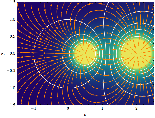
Here is an example of how to use the function. The contour lines of the potential are shown in white, and the streamlines of the gradient field are orange.
gradientFieldPlot[
(y^2 + (x - 2)^2)^(-1/2) - (y^2 + (x - 1/2)^2)^(-1/2)/2,
{x, -1.5, 2.5}, {y, -1.5, 1.5},
 PlotPoints -> 50, ColorFunction -> "BlueGreenYellow", Contours -> 10,
  ContourStyle -> White, Frame -> True, FrameLabel -> {"x", "y"},
 ClippingStyle -> Automatic, Axes -> True, StreamStyle -> Orange]
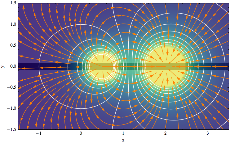
But perhaps you would like to emphasize the horizontal axis by making it really thick. Now you can achieve this without obscuring the plot:
gradientFieldPlot[(y^2 + (x - 2)^2)^(-1/
   2) - (y^2 + (x - 1/2)^2)^(-1/2)/2, {x, -1.5, 3.5}, {y, -1.5, 1.5},
 PlotPoints -> 50, ColorFunction -> "BlueGreenYellow", Contours -> 16,
  ContourStyle -> White, Frame -> True, FrameLabel -> {"x", "y"},
 ClippingStyle -> Automatic, StreamStyle -> Orange, ImageSize -> 500,
 GridLinesStyle -> Directive[Thick, Black], "ShadingOpacity" -> .8,
 Axes -> {True, False}, AxesStyle -> Directive[Thickness[.03], Black],
  Method -> {"AxesInFront" -> False}]